Field Detail

• scale

  private double scale

  Reference: Statistical Distributions Fourth Edition, Catherine Forbes, Merran Evans, Nicholas Hastings, and Brian Peacock, Chqapter 46, Weibull Distribution, pp. 193-201. Variable 0 = 0 is the characteristic life shape parameter > 0 0 0 for 2 parameters pdf: 0 for t location for 3 parameters pdf: 0 for t location = 0 for t The aim of this package is to provide state of the art tools for all kinds of Weibull analyses.
  The license follows: MIT License Copyright (c) 2020-present Tamer Tevetoglu Permission is hereby granted, free of charge, to any person obtaining a copy of this software and associated documentation files (the "Software"), to deal in the Software without restriction, including without limitation the rights to use, copy, modify, merge, publish, distribute, sublicense, and/or sell copies of the Software, and to permit persons to whom the Software is furnished to do so, subject to the following conditions: The above copyright notice and this permission notice shall be included in all copies or substantial portions of the Software. THE SOFTWARE IS PROVIDED "AS IS", WITHOUT WARRANTY OF ANY KIND, EXPRESS OR IMPLIED, INCLUDING BUT NOT LIMITED TO THE WARRANTIES OF MERCHANTABILITY, FITNESS FOR A PARTICULAR PURPOSE AND NONINFRINGEMENT. IN NO EVENT SHALL THE AUTHORS OR COPYRIGHT HOLDERS BE LIABLE FOR ANY CLAIM, DAMAGES OR OTHER LIABILITY, WHETHER IN AN ACTION OF CONTRACT, TORT OR OTHERWISE, ARISING FROM, OUT OF OR IN CONNECTION WITH THE SOFTWARE OR THE USE OR OTHER DEALINGS IN THE SOFTWARE. You can cite predictr in your publication or research work using the Digital Object Identifier (DOI): 10.5281/zenodo.4614034 ## BibTeX

• shape

  private double shape

• location

  private double location

• w

  private double[] w

• t

  private double[] t

• n

  private int n

• UI

  private ViewUserInterface UI

• failures

  private double[] failures

• suspensions

  private double[] suspensions

Constructor Detail

• WeibullDistribution

  public WeibullDistribution()

• WeibullDistribution

  public WeibullDistribution​(double scale,
                             double shape,
                             double location,
                             double[] w,
                             double[] t)

Method Detail

• generateRandomWeibull2param

  public void generateRandomWeibull2param()

• generateRandomWeibull3param

  public void generateRandomWeibull3param()

• generateSequentialWeibull2param

  public void generateSequentialWeibull2param()

• generateSequentialWeibull3param

  public void generateSequentialWeibull3param()

• testSequentialWeibull2param

  public void testSequentialWeibull2param()

• testSequentialWeibull3param

  public void testSequentialWeibull3param()

• testInitialThreeParameterApproximation

  public void testInitialThreeParameterApproximation()

• intialThreeParameterApproximation

  public void intialThreeParameterApproximation​(double[] scale0,
                                                double[] shape0,
                                                double[] location0)

• testRandomWeibull

  public void testRandomWeibull()

• fitToExternalFunction

  public boolean fitToExternalFunction​(double[] x,
                                       double[] residuals,
                                       double[][] jacobian)

  Specified by:

  fitToExternalFunction in class CeresSolver

• test_mle

  public void test_mle()

  Maximum likelihood estimation (MLE):** ```python from predictr import Analysis prototype_a = Analysis(...) # create an instance prototype_a.mle() # use instance methods ``` Median Rank Regression (MRR)** ```python from predictr import Analysis prototype_a = Analysis(...) # create an instance prototype_a.mrr() # use instance methods ``` ### Bias-correction methods Since parameter estimation methods are only asymptotically unbiased (sample sizes -> "infinity"), bias-correction methods are useful when you have only a few failures. These methods correct the Weibull shape and scale parameter. The following table provides possible configurations. Bias-corrections for mrr() are not supported, yet.
  | Bias-correction method | mle() | mrr() | argument value | config. | statistic | |-------------------------------------|:-----:|:-----:|:--------------:|:-------:|:--------------------------------:| | C4 aka 'reduced bias adjustment' | x | - | 'c4' | - | - | | Hirose and Ross method | x | - | 'hrbu' | - | - | | Non-parametric Bootstrap correction | x | - | 'np_bs' | bs_size | 'mean', 'median', 'trimmed_mean' | | Parametric Bootstrap correction | x | - | 'p_bs' | bs_size | 'mean', 'median', 'trimmed_mean' | ### Confidence bounds methods Analysis supports nearly all state of the art confidence bounds methods. | confidence bounds | mle() | mrr() | uncensored data | censored data | bounds_type | argument value | |---------------------------------|:-----:|:-----:|:---------------:|:-------------:|:------------------:|:--------------:| | Beta-Binomial Bounds | - | x | x | x | '2s', '1sl', '1su' | 'bbb' | | Monte-Carlo Pivotal Bounds | - | x | x | x | '2s', '1sl', '1su' | 'mcpb' | | Non-Parametric Bootstrap Bounds | x | x | x | x | '2s', '1sl', '1su' | 'npbb' | | Parametric Bootstrap Bounds | x | x | x | x | '2s', '1sl', '1su' | 'pbb' | | Fisher Bounds | x | - | x | x | '2s', '1sl', '1su' | 'fb' | | Likelihood Ratio Bounds | x | - | x | x | '2s', '1sl', '1su' | 'lrb' | Important**: - mle() and mrr() support only specific confidence bounds methods. For instance, you can't use Beta-Binomial Bounds with mle(). This will also raise an error. Use the table above to check, whether a combination of parameter estimation and confidence bounds method is supported. - '2s': two-sided confidence bounds, '1su': upper confidence bounds, '1sl': lower confidence bounds. If Beta-Binomial Bounds are used, the lower bound represents the lower percentile bound at a specific time ((pctl) is added in the plot legend). If Fisher Bounds are used, the lower bound represents the lower time bound at a specific percentile. ### Examples #### Maximum Likelihood Estimation (MLE) ##### Uncensored sample Example: ```python failures = [0.4508831, 0.68564703, 0.76826143, 0.88231395, 1.48287253, 1.62876357] prototype_a = Analysis(df=failures, bounds='fb',show=True) prototype_a.mle() ``` 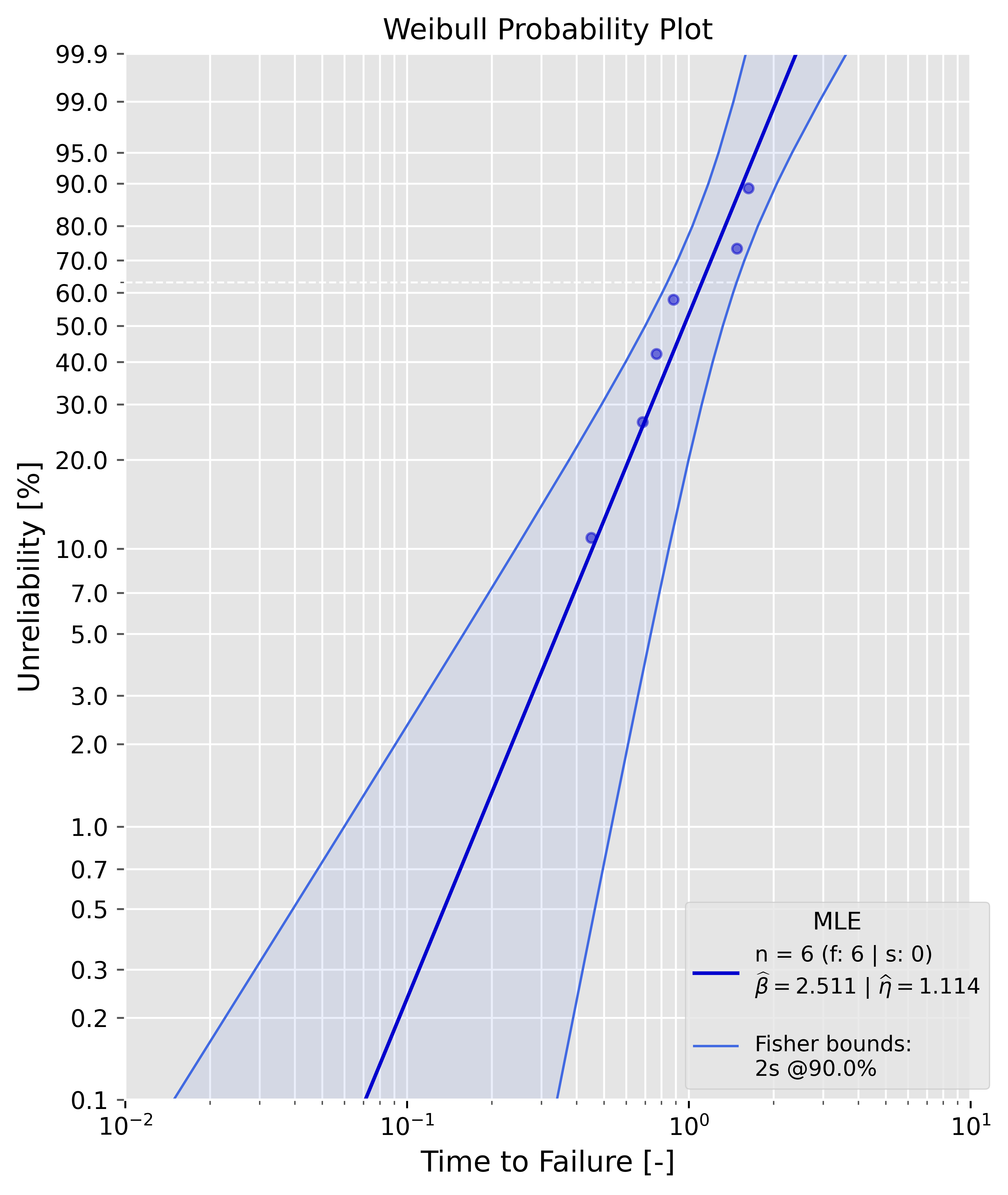{: width="500" } ##### Censored sample Example: ```python failures = [0.4508831, 0.68564703, 0.76826143, 0.88231395, 1.48287253, 1.62876357] suspensions = [1.9, 2.0, 2.0] prototype_a = Analysis(df=failures, ds=suspensions, bounds='lrb',show=True) prototype_a.mle() ``` 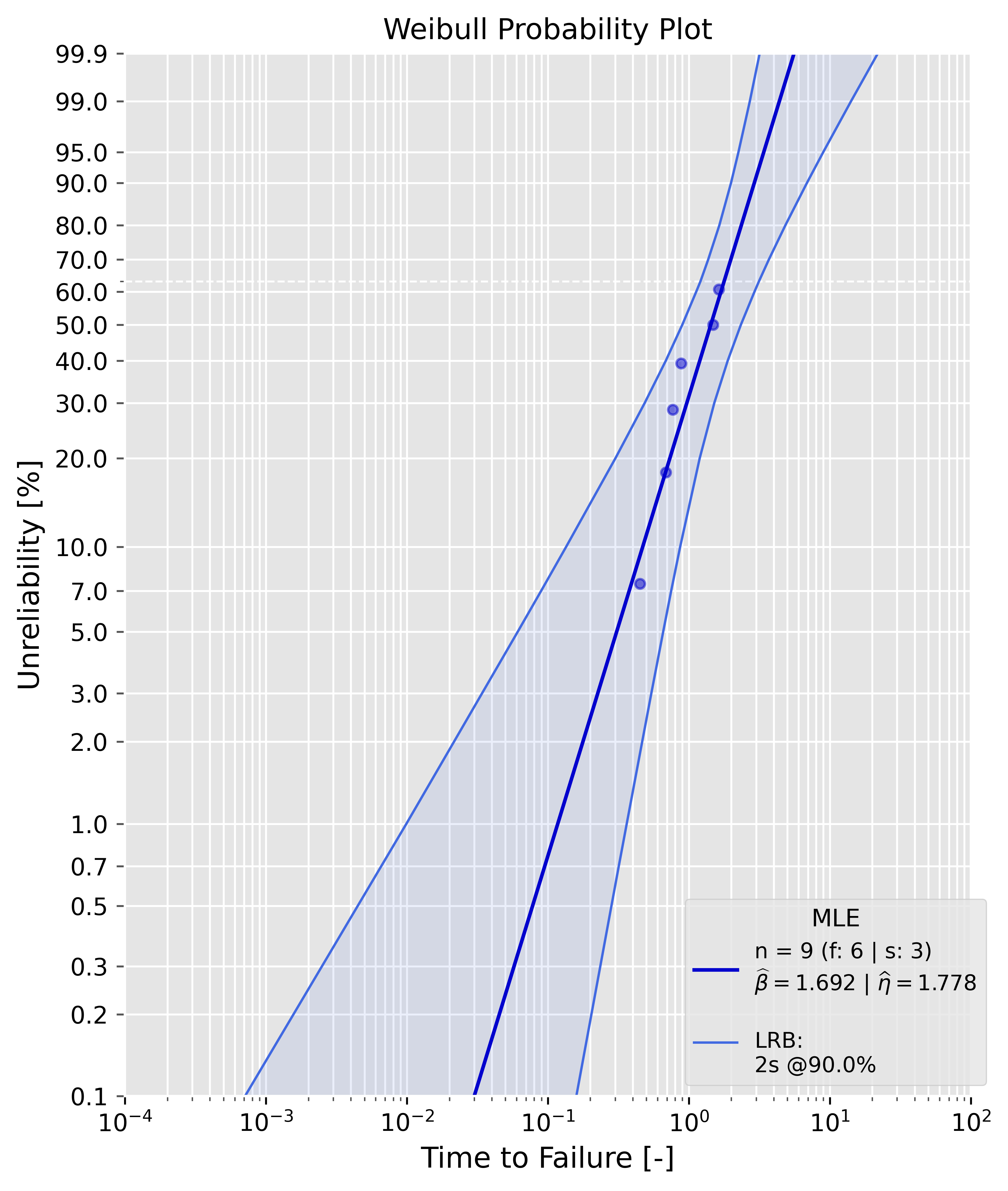{: width="500" } #### Median Rank Regression (MRR) ##### Uncensored sample Example: ```python failures = [0.4508831, 0.68564703, 0.76826143, 0.88231395, 1.48287253, 1.62876357] prototype_a = Analysis(df=failures, bounds='bbb',show=True) prototype_a.mrr() ``` 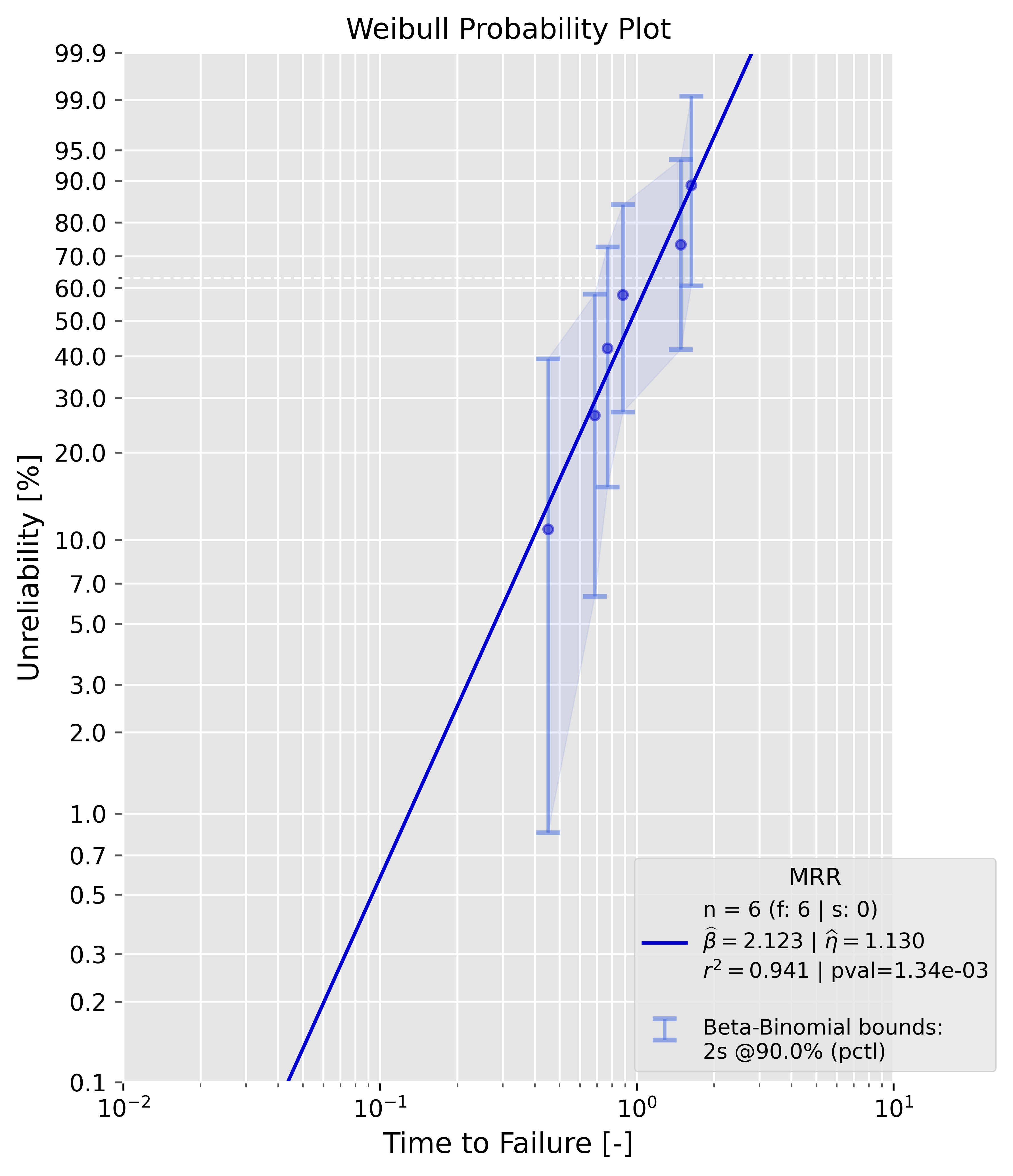{: width="500" } ##### Censored sample Example: ```python failures = [0.4508831, 0.68564703, 0.76826143, 0.88231395, 1.48287253, 1.62876357] suspensions = [1.9, 2.0, 2.0] prototype_a = Analysis(df=failures, ds=suspensions, bounds='mcpb',show=True) prototype_a.mrr() ##### Censored sample Example: ```python failures = [0.4508831, 0.68564703, 0.76826143, 0.88231395, 1.48287253, 1.62876357] suspensions = [1.9, 2.0, 2.0] prototype_a = Analysis(df=failures, ds=suspensions, bounds='mcpb',show=True) prototype_a.mrr() ``` 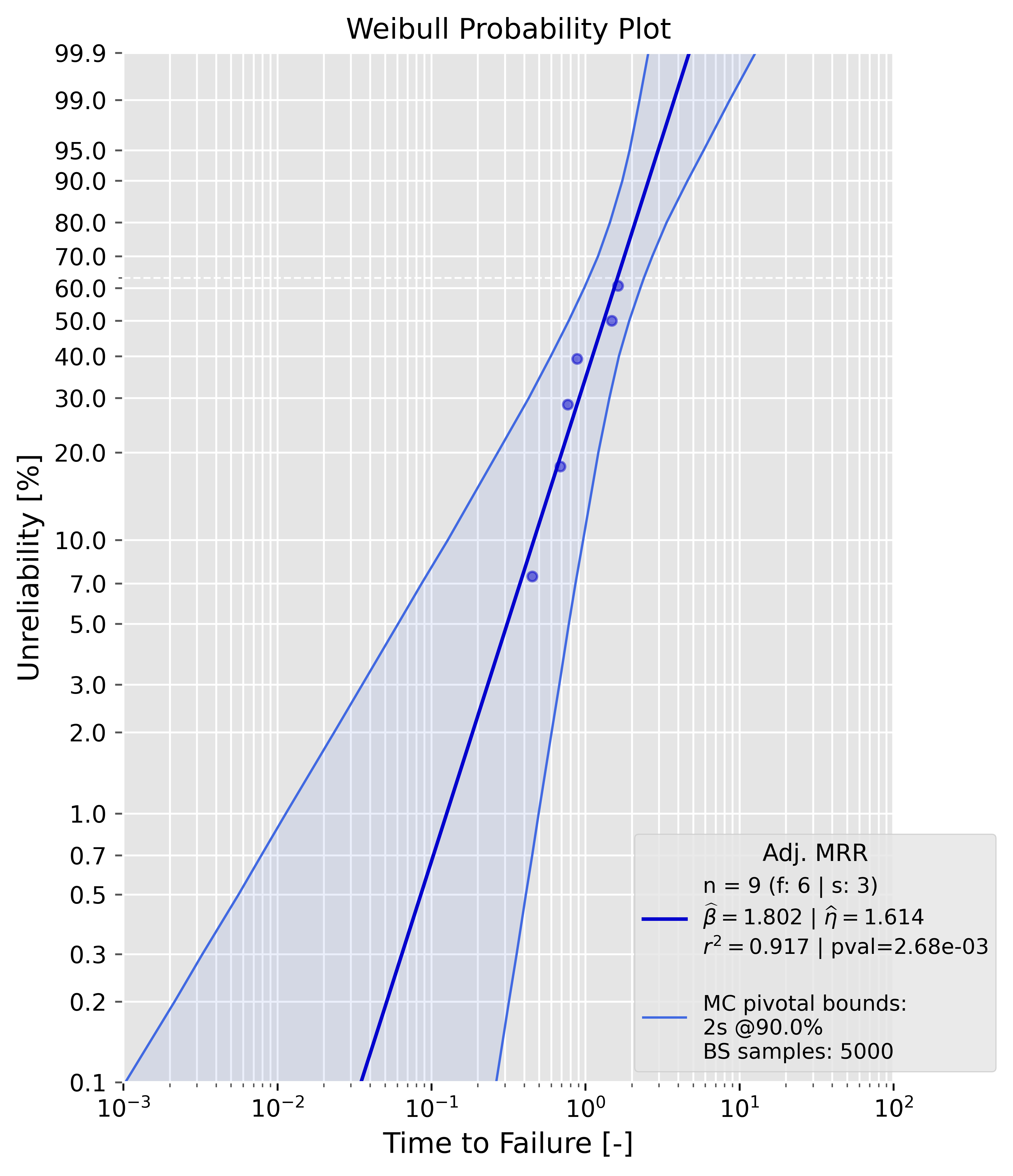{: width="500" } #### Bias-corrections As already mentioned, only mle() support bias-corrections. The samples in these examples are drawn from a two-parameter Weibull distribution with a shape parameter of 2.0 and a scale parameter of 1.0. ##### Uncensored sample It is appearent that the estimates of beta and eta are now closer to the ground truth values. The dotted grey line in the plot is the "biased" MLE line, the bia-corrected line is blue. The legend contains all needed information. ```python failures = [0.4508831, 0.68564703, 0.76826143, 0.88231395, 1.48287253, 1.62876357] prototype_a = Analysis(df=failures, bounds='fb', show=True, bcm='c4') prototype_a.mle() ``` 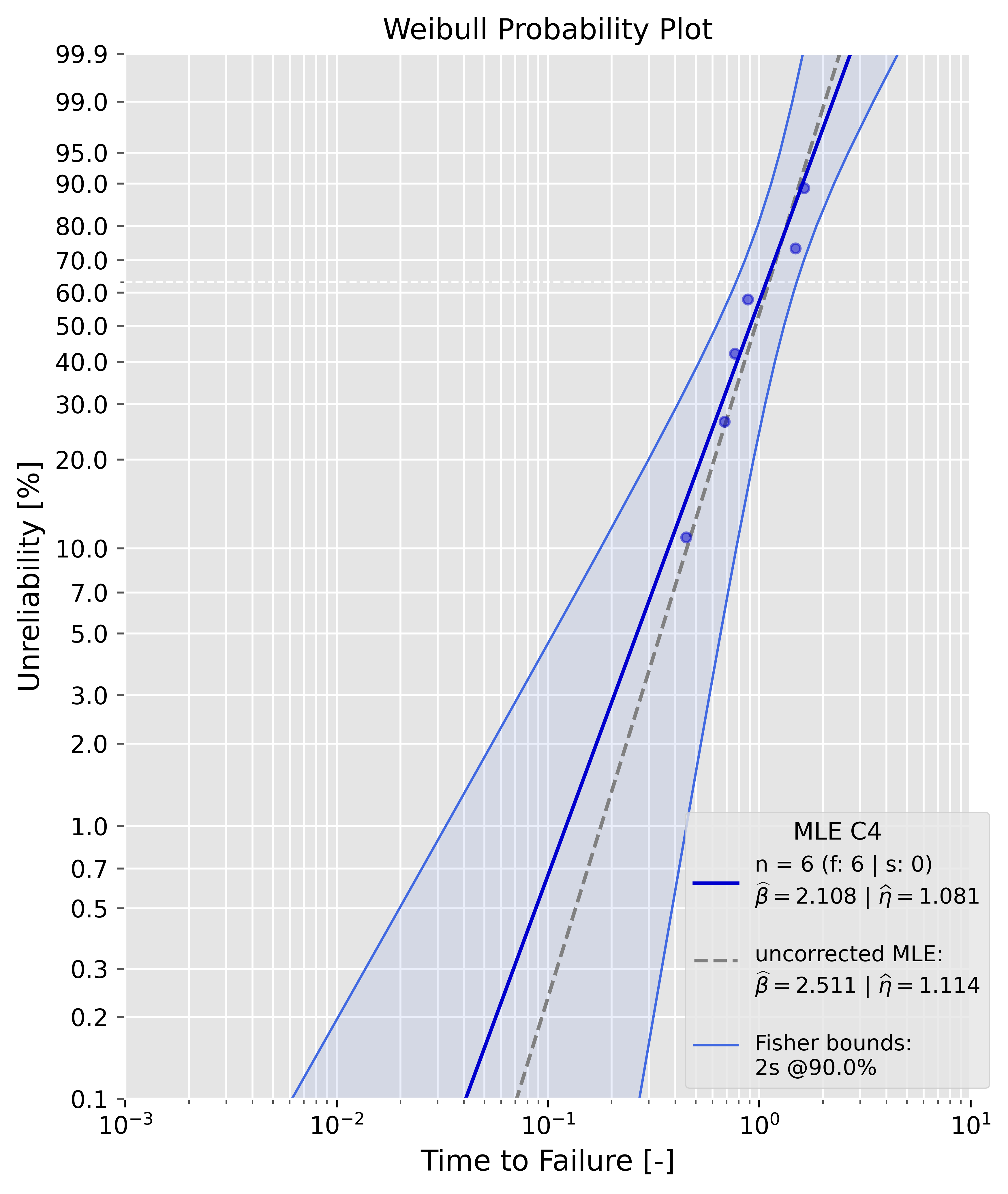{: width="500" } The estimates can for the Weibull parameters can be compared directly, since they are available as attributes ```python print(f'biased beta: {prototype_a.beta:4f} --> bias-corrected beta: {prototype_a.beta_c4:4f}') >>> biased beta: 2.511134 --> bias-corrected beta: 2.108248 ``` ##### Censored sample The data is type II right-censored. ```python failures = [0.38760099164906514, 0.5867052007217437, 0.5878056753744406, 0.602290402929083, 0.6754829518358306, 0.7520219855697948] suspensions = [0.7520219855697948, 0.7520219855697948] prototype_a = Analysis(df=failures, ds=suspensions, bounds='lrb', show=True, bcm='hrbu') prototype_a.mle()

• test_mrr

  public void test_mrr()