Fast Fourier Transformation (FFT)

There are two main approaches to filtering an image. The first is the convolution of an image and kernel in the spatial domain. The second is the multiplication of an image's Fourier transform with a filter in the frequency domain. The Fast Fourier transformation (FFT) algorithm, which is an example of the second approach, is used to obtain a frequency-filtered version of an image. Processing images by filtering in the frequency domain is a three-step process:

1. Perform a forward fast Fourier transform to convert a spatial image to its complex fourier transform image. The complex image shows the magnitude frequency components. It does not display phase information.
2. Enhance selected frequency components of the image and attenuate other frequency components of the image by multiplying by a low-pass, high-pass, band-pass, or band-stop filter. In MIPAV, you can construct frequency filters using one of three methods: finite impulse response filters constructed with Hamming windows, Gaussian filters, and Butterworth filters. However, for the Gaussian filters, only low-pass and high-pass filters are available.
3. Perform an inverse fast fourier transform to reconvert the image from the frequency domain to the spatial domain.

You can also use Algorithms > Filters (frequency) to obtain a frequency-filtered version of an image in a single step. A contrast of the FFT and Filter (frequency) commands on the Algorithms menu is helpful in determining which one to select.

Fast Fourier Transformation (FFT) algorithm:background;

Since all dimensions of an n-dimensional dataset must be powers of 2, datasets with arbitrary dimensions are zero padded to powers of 2 before applying the Fast Fourier Transform and stripped down to the original dimensions after applying the Inverse Fast Fourier Transform.

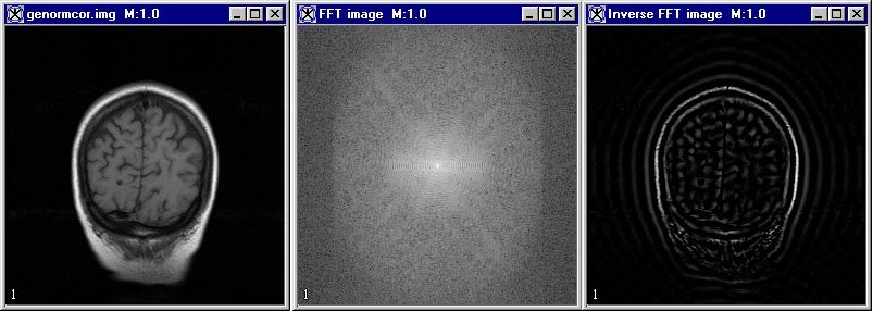
If real source data is used, then the output obtained after the final Inverse Fast Fourier Transform step is purely real, no matter what filter construction method is used. Any non-zero imaginary part present after the Inverse Fast Fourier Transform is due to Randolph error. Hence, the imaginary part is discarded and only the real part is imported into the final image. Figure 1 shows the application of the FFT algorithm to a 2D image.

Figure 1. FFT algorithm processing

In MIPAV, frequency filters may be constructed using one of three methods: finite impulse response filters constructed with Hamming windows, Gaussian filters, and Butterworth filters. You select the method when you enter the parameters for the algorithm.

If you use FIR filters with Hamming windows, an ideal filter kernel is constructed in the spatial domain. A Hamming window kernel is also constructed in the spatial domain. Then, the ideal filter kernel and the Hamming window kernel are multiplied together in the spatial domain. The resultant kernel is a circle or odd diameter sphere with its center at (kernel diameter - 1)/2 in every dimension. The kernel is zero padded up to the same dimensions as the original image data.

The two fourier transforms (image and filter) are multiplied, and the inverse fourier transform is obtained. The result is a filtered version of the original image shifted by (kernel diameter - 1)/2 toward the end of each dimension. The data is shifted back by (kernel diameter - 1)/2 to the start of each dimension before the image is stripped to the original dimensions.

In every dimension the length of the resulting fourier image must be greater than or equal to the length of non-zero image data kernel diameter - 1 so that aliasing does not occur. In aliasing, higher frequency components incorrectly shift to lower frequencies. Thus, if the image is not cropped, each frequency space dimension must be greater than or equal to the minimum power of two that equals or exceeds the original dimension size kernel diameter 1. If cropping is selected, the fourier image is only increased to the minimum power of 2 that equals or exceeds the original dimension size rather than the minimum power 2 that equals or exceeds the original dimension size kernel diameter - 1. With cropping, a band of pixels at the boundaries of the image is set equal to 0. A power of 2 increase in dimension length is avoided at the cost of losing edge pixels.

The following formula defines the discrete-space fourier transform pair:

${\displaystyle X({\omega }_1,{\omega }_2)={\displaystyle \sum _{n_1=-\mathrm{\infty }}^{\mathrm{\infty }}}{\displaystyle \sum _{n_2=-\mathrm{\infty }}^{\mathrm{\infty }}}x(n_1,n_2)e^{-j{\omega }_1{n}_1}{e}^{-j{\omega }_2{n}_2}}$

${\displaystyle x(n_1{n}_2)=\frac{1}{(2\pi {)}^2}{\displaystyle \underset{{\omega }_1}{\overset{\pi }{\int }}}=-\pi {\displaystyle \underset{w_2}{\overset{\pi }{\int }}}=-{\pi }^{X({\omega }_1,{\omega }_2)e^{-j{\omega }_1{n}_1}{e}^{-j{\omega }_2{n}_2}}\partial {\omega }_1\partial {\omega }_2}$

While centering is invoked in FFT to provide a clearer display, centering is not used in frequency filter where no fourier images are produced.

In the frequency filtering step, both the real and imaginary parts of the fourier transform are scaled by the same formula, which depends only on the distance from the center of image.

The FIR filter must create two fourier transforms: one for the original image and one for the kernel. The Butterworth and Gaussian filters only need to create one fourier transform for the image since frequency scaling is done with a formula. Therefore, the FIR filter uses about twice as much memory as the Gaussian or Butterworth filters.

Centering is needed for the Gaussian and Butterworth filters since the scaling formulas are based on frequency magnitude increasing from the center of the image.

• • Butterworth filters:2D;
    
  • Butterworth filters:3D;
    

The following are the formulas for the Butterworth 2D and 3D filters, respectively.'

${\displaystyle distsq=\frac{(x-xcenter{)}^2}{(xcenter{)}^2}+\frac{(y-ycenter{)}^2}{(ycenter{)}^2}}$

${\displaystyle distsq=\frac{(x-xcenter{)}^2}{(xcenter{)}^2}+\frac{(y-ycenter{)}^2}{(ycenter{)}^2}+\frac{(z-zcenter{)}^2}{(zcenter{)}^2}}$

The real data is the product of the real data and the coefficient. The imaginary data is the product of the imaginary data and the coefficient.

• • Butterworth filters:high-pass;
    
  • Butterworth filters:low-pass;
    
  • Butterworth filters:band-stop;
    
  • Butterworth filters:band-stop;
    

The following are the equations for the Butterworth low-pass, high-pass, band-pass, and band-stop filters.

${\displaystyle coefficient=\frac{1}{1+{\left(\frac{distsq}{(f_1)}\right)}^{2butterworthorder}}}$

${\displaystyle coefficient=\frac{1}{1+{\left(\frac{(f_1)}{distsq}\right)}^{2butterworthorder}}}$

${\displaystyle width=f_2-f_{1}centersq=f_1{f}_2}$

${\displaystyle num=(distsq-centersq{)}^{2butterworthorder}}$

${\displaystyle coeff=\frac{num}{(num+(distsq-centersq{)}^{2butterworthorder})}}$

${\displaystyle width=f_2=f_1,centersq=f_1{f}_2}$

${\displaystyle num=(\sqrt{d}istsqwidth{)}^{2butterworthorder}}$

${\displaystyle coeff=\frac{num}{(num+(\sqrt{d}istsqwidth{)}^{2butterworthorder})}}$

The following equations are for the Gaussian low- and high-pass filters.

${\displaystyle coefficientforgaussianhighpass=1-gaussianlowpass}$

${\displaystyle coefficient=e^{-\frac{(x-xcenter{)}^2}{(2f^{2}xcente{r}^2)}}{e}^{-\frac{(y-ycenter{)}^2}{(2f^{2}ycente{r}^2)}}{e}^{-\frac{(z-zcenter{)}^2}{(2f^{2}zcente{r}^2)}}}$

• • i.routine bessj1;
    

• • Fast Fourier Transformation (FFT) algorithm:image types;
    
  • image types:Fast Fourier Transformation (FFT) algorithm;
    

You cannot apply a forward FFT to complex data. However, you can apply the frequency filter or perform an inverse FFT on conjugate, symmetric, and complex data. You cannot apply this algorithm to Alpha Red Green Blue (ARGB) datasets, but you can apply it to other gray-scale 2D and 3D images.

By default, the resultant image is a float-type image. Intermediate fourier transform images and filtered fourier transform images obtained in FFT are complex images.

• • Fast Fourier Transformation (FFT) algorithm:references ;
    

Refer to the following references for more information about this algorithm:

Nasir. Ahmed, Discrete-Time Signals and Systems (Reston, Virginia: Reston Publication Company, 1983), pp. 243-258.

Raphael C. Gonzalez and Richard E. Woods. Digital Image Processing (Boston: Addison-Wesley, 1992), pp. 201-213, 244.

Jae S. Lim and Joe S. Lim, Two-Dimensional Signal and Image Processing (Upper Saddle River, New Jersey: Prentice-Hall PTR, 1990), pp. 57-58, 195-213.

William H. Press, Brian P. Flannery, Saul A. Teukolsky, and William T. Vetterling, "Numerical Recipes in C," The Art of Scientific Computing, Second Edition (Cambridge, Massachusetts: Cambridge University Press, p. 1993), pp. 233, 521-525.

• • Fast Fourier Transformation (FFT) algorithm:applying;
    
  • applying:FFT algorithm;
    

Generally, when an image is filtered in the frequency domain, you use the following three-step process:

1. Apply Forward FFT. In this first step, the spatial image is converted to a complex fourier transform image.
2. Apply Frequency Filter: Next, you can enhance and attenuate selected frequency components by multiplying the fourier transform image by the low-pass, high-pass, band-pass, or band-stop filters.
3. Apply Inverse FFT: Finally, you can perform an inverse fast fourier transform to reconvert the image to the spatial domain.

You can use the FFT algorithm to perform one or all of these steps.

• • commands:format FFT;
    
  • converting dataset from spatial to fourier domain;
    
  • forward FFT command;
    
  • image dataset:converting from spatial to fourier domain;
    

To convert the dataset from the spatial to fourier domain, complete the following steps:

1. In the Default Image window, open a dataset that is displayed in the spatial domain.
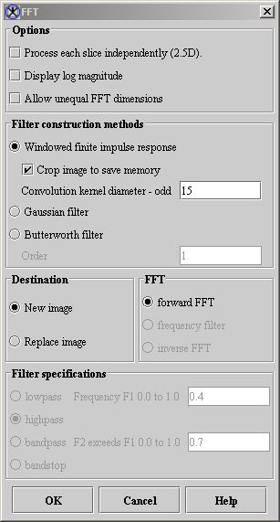
2. In the MIPAV window, select Algorithm > FFT. The FFT dialog box opens (Figure 2).
3. Select the destination.
4. By default, the forward FFT is selected. (The frequency filter and inverse FFT methods cannot be applied to real spatial datasets.)
5. Select the filter construction method. If you select the Butterworth filter, enter the order.
   • FIR: Click Windowed finite impulse response. Enter the kernel diameter, which must be an odd number that is greater than or equal to 3. To save memory at the expense of zeroing edge pixels, select or clear image cropping.
   • Gaussian: Click Gaussian filter.
   • Butterworth: Click Butterworth filter, and then enter the order of the Butterworth filter.
6. Having selected the filter construction method, you can choose to apply the following options:
   • If you select Display log magnitude, the log10 [1 square root (real part**2 imaginary part**2)] is shown. If the Display log magnitude is clear, square root (real part**2 imaginary part**2) is shown.
   • If your image has unequal dimensions, you can select Allow unequal FFT dimensions to allow unequal FFT dimensions. If you want the FFT to equalize the dimensions to produce a symmetrical image, clear the check box.
   • If you selected the FIR filter, you can crop the image to save memory. Enter an odd number for the convolution kernel diameter. The number must be odd so there is symmetry around a center point.
7. Click OK to perform the forward FFT. MIPAV applies the FFT algorithm. When complete, the fourier transform of the image appears.

• • frequency components:enhancing and attenuating ;
    
  • enhancing and attenuating frequency components;
    

To apply the frequency option to enhance and attenuate frequency components, complete the following steps:

1. Select the fourier transform of a spatial image. The image appears in a default image window.
2. In the MIPAV window, select Algorithms > FFT. The FFT dialog box (Figure 2) opens.
3. Select the destination.
4. Select Frequency Filter.
5. Click, if desired, the check box to display the log magnitude.
6. Select one of the following filter specifications:
   • Lowpass: Type the value of the frequency. The value must be greater than 0.0, but less than or equal to 1.0. where 0.0 is the zero frequency and 1.0 is the absolute value of the frequency at the end of a centered fourier dimension.
   • Highpass: Enter the value of the frequency. The value must be greater than 0.0, but less than or equal to 1.0. 0.0 is the zero frequency, 1.0 is the absolute value of the frequency at the end of a centered fourier dimension.
   • Bandpass: Type the values of the frequencies F1 and F2, with F2 greater than F1. The value must be greater than 0.0, but less than or equal to 1.0 where 0.0 is the zero frequency and 1.0 is the absolute value of the frequency at the end of a centered fourier dimension.
   • Bandstop: Enter the values of the frequencies F1 and F2, with F2 greater than F1. The value must be greater than 0.0, but less than or equal to 1.0 where 0.0 is the zero frequency and 1.0 is the absolute value of the frequency at the end of a centered fourier dimension.
7. When complete, click OK. MIPAV applies the FFT algorithm. When complete, the fourier transform of the image appears.

Figure 2. FFT dialog box

Process each slice independently (2.5D)	Filters each slice of the dataset independently of adjacent slices.
Display log magnitude	Displays 1 plus the magnitude of the FFT.
Allow unequal FFT dimensions	Allows the image to have unequal dimensions. If this option is not selected, FFT makes the dimensions equal, which may result in more memory usage during processing.
Windowed finite impulse response	Constructs an ideal filter kernel and a Hamming window kernel in the spatial domain and multiplies them. The resultant kernel is a circle or sphere of odd diameter with its center at (kernel diameter -1)/2 in every dimension.
Crop image to save memory	Saves memory by assigning the edge pixels of the image a value of zero.
Convolution kernel diameter-odd	Limits the diameter of the convolution kernel to the size that you specify.
Gaussian filter	Applies the Gaussian filter to the image. The Gaussian filters only low-pass and high-pass filters are available.
Butterworth filter	Applies the Butterworth filter, which has a maximally flat response in its passband. The passband is the range of frequencies that pass with a minimum of attenuation through an electronic filter.
Order	Displays the order of the Butterworth filter.
New image	Places the result of the algorithm in a new image window.
Replace image	Replaces the current active image with the results of the algorithm.
Forward FFT	Converts spatial image to a complex fourier transform image.
Frequency filter	Enhances or attenuates selected frequency components by multiplying the fourier transform image by the low-pass, high-pass, band-pass, or band-stop filters.
Lowpass	Suppresses frequencies above a specified threshold. Frequencies below the threshold are transmitted.
Highpass	Suppresses frequencies below a specified threshold. Frequencies above the threshold are transmitted.
Bandpass	Suppresses all frequencies except those in a specified band.
Bandstop	Suppresses a band of frequencies from being transmitted through the filter. Frequencies above and below the band are transmitted.
OK	Applies the FFT algorithm according to the specifications in this dialog box.
Cancel	Disregards any changes that you made in this dialog box and closes the dialog box.
Help	Displays online help for this dialog box.

With the Paint tool you can attenuate frequency components to values whose magnitude is 1,000 times the minimum floating point value. The values are not simply attenuated to zero because this would result in the phase information being lost and cause phase discontinuities in the image. Frequency components whose magnitudes are less than or equal to 1,000 times the minimum floating point value are unaffected by the paint tool. To do this, complete the following steps:

1. Display the paint toolbar if it is not already visible. To do this, in the MIPAV window, select Toolsbar > Paint toolbar. The paint toolbar appears.
2. Select Paint Brush to select the paint brush.
3. Select the size of the paint brush tip. Choose one of the following:
   • Small Tip-To select a tip that is one pixel in size.
   • Medium Tip-To select a tip that is 16 pixels (4 x 4 square) in size.
   • Large Tip-To select a tip that is 100 pixels (10 x 10 square) in size. As you draw, you can select one pixel at a time or drag to draw paint strokes on the image.

As you draw, you can select one pixel at a time or drag to draw paint strokes on the image.

• • conjugate symmetric fourier transform;
    
  • image:complex, mirroring technique used in drawing;
    

1. When finished, to return to normal mode, click Normal Mode.
2. You can erase the paint from the image's paint layer by completing the following steps. You can either erase all paint from the image or erase paint from a specific conjugate symmetric area.

To erase all paint in the image, click Global Erase.

To erase space from a specific area, complete the following steps

• Click Erase.
• Select the size of the eraser tip. Click Small Tip to select a tip that is 1 pixel in size. Click Medium Tip to select a tip that is 16 pixels (4 x 4 square) in size. Click Large Tip to select a tip that is 100 pixels (10 x 10 square) in size.
• Use the mouse to begin erasing. You can select one pixel at a time or drag the mouse. If desired, use the magnification buttons to magnify the image.
• When finished, to return to normal mode, click Normal Mode.

1. Click Commit to commit the changes (copy them permanently to an image).

To reconvert the image to the spatial domain, complete the following steps:

1. Select the fourier transform of a spatial image. The image appears in a default image window.
2. In the MIPAV window, select Algorithms > FFT. The FFT dialog box
   (Figure 2) opens.
3. Select the destination.
4. Select Inverse FFT.
5. If desired, click Display log magnitude.
6. Click OK. When complete processing is complete, the image appears in the spatial domain.

• Using MIPAV Algorithms
  • Cost functions used in MIPAV algorithms
  • Interpolation methods used in MIPAV
  • Degrees of freedom
  • Filters (Spatial): Adaptive Noise Reduction
  • Filters (Frequency)
  • Filters (Spatial): Adaptive Path Smooth
  • Filters (Spatial) Anisotropic Diffusion
  • Filters (Spatial): Coherence-Enhancing Diffusion
  • Filters (Spatial): Gaussian Blur
  • Filters (Spatial): Gradient Magnitude
  • Filters (Spatial) Laplacian
  • Filters (Spatial) Local Normalization
  • Filters (Spatial): Mean
  • Filters (Spatial): Median
  • Filters (Spatial): Mode
  • Filters (Spatial): Nonlinear Noise Reduction
  • Filters (Spatial): Nonmaximum Suppression
  • Filters (Spatial): Regularized Isotropic (Nonlinear) Diffusion
  • Filters (Spatial): Slice Averaging
  • Filters (Spatial): Unsharp Mask
  • Filters (Wavelet): Thresholding