Filters (Spatial): Gaussian Blur

This algorithm blurs an image or the VOI of the image with a Gaussian function at a user-defined scale sigma (standard deviation [SD]). In essence, convolving a Gaussian function produces a similar result to applying a low-pass or smoothing filter. A low-pass filter attenuates high-frequency components of the image (i.e., edges) and passes low-frequency components. This results in the blurring of the image. Smoothing filters are typically used for noise reduction and for blurring. The standard deviation of the Gaussian function controls the amount of blurring. A large standard deviation (i.e., > 2) significantly blurs, while a small standard deviation (i.e., 0.5) blurs less. If the objective is to achieve noise reduction, a rank filter (median) might be more useful in some circumstances.

Advantages to convolving the Gaussian function to blur an image include:

Structure is not added to the image.
It, as well as the Fourier Transform of the Gaussian, can be analytically calculated.
By varying the SD, a Gaussian scale space can easily be constructed.

Background

The radially symmetric Gaussian, in an n-dimensional space, is:'

Equation 10

where (referred to as the scale), is the standard deviation of the Gaussian and is a free parameter that describes the width of the operator (and thus the degree of blurring) and n indicates the number of dimensions.

Geometric measurements of images can be obtained by spatially convolving (shift-invariant and linear operation) a Gaussian neighborhood operator with an image, I, where represents an n-dimensional image. The convolution process produces a weighted average of a local neighborhood where the width of the neighborhood is a function of the scale of the Gaussian operator. The scale of the Gaussian controls the resolution of the resultant image and thus the size of the structures that can be measured. A scale-space for an image of increasingly blurred images can be defined by L:nx and where represents convolution.

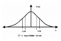
The following is the calculation of the full-width half max (FWHM) of the Gaussian function.


$G (x, σ) = \frac{1}{\sqrt{2 π σ^{2}}} e^{- \frac{x^{2}}{2 σ^{2}}}$ $l n 0.5 \frac{1}{\sqrt{2 π σ^{2}}} = l n (\frac{1}{\sqrt{2 π σ^{2}}} e^{- \frac{x^{2}}{2 σ^{2}}})$ $l n 0.5 + l n (\frac{1}{\sqrt{2 π σ^{2}}}) = l n (\frac{1}{\sqrt{2 π σ^{2}}}) + l n (e^{- \frac{x^{2}}{2 σ^{2}}})$ $- 0.693 = - \frac{x^{2}}{2 σ^{2}}$ $1.18 σ = x$

Figure 2 shows the Gaussian function. The dotted lines indicate the standard deviation of 1. The FWHM is indicated by the solid lines. For a Gaussian with a standard deviation equal to 1 (), the FWHM is 2.36.

**Figure 1. Gaussian Blur algorithm processing**

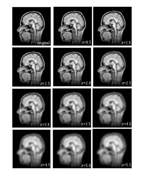Figure 1 shows a Gaussian scale-space of the sagittal view of a MR head image. The original image is shown in the upper left (). Varying s from 0.5 to 5.5 in steps of 0.5 blurs the other images (from left to right and top to bottom).

**Figure 2. Gaussian function**

Note that as the scale increases, small-scale features are suppressed. For example, at small scales the individual folds of the brain are quite defined, but, as the scale increases, these folds diffuse together resulting in the formation of a region one might define as the brain.

Image types

You can apply this algorithm to all image data types except Complex and to 2D, 2.5D, 3D, and 4D images.

By default, the resultant image is a float type image.
By selecting Process each slide independently (2.5D) in the Gaussian Blur dialog box, you can achieve 2.5D blurring (each slice of the volume is blurred independently) of a 3D dataset (Figure 1).

Special notes

None.

References

See the following references for more information about this algorithm:

J. J. Koenderink, "The Structure of Images," Biol Cybern 50:363-370, 1984.

J. J. Koenderink and A. J. van Doorn, "Receptive Field Families," Biol Cybern 63:291-298, 1990.

Tony Lindeberg, "Linear Scale-Space I: Basic Theory," Geometry-Driven Diffusion in Computer Vision, Bart M. Ter Har Romeney, ed. (Dordrecht, The Netherlands: Kluwer Academic Publishers, 1994), pp. 1-38.

R. A. Young, "The Gaussian Derivative Model for Machine Vision: Visual Cortex Simulation," Journal of the Optical Society of America, GMR-5323, 1986.

Applying the Gaussian Blur algorithm

To run this algorithm, complete the following steps:

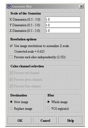
Select Algorithms > Filter > Gaussian Blur. The Gaussian Blur dialog box opens (Figure 3).
Complete the information in the dialog box.
Click OK.

The algorithm begins to run, and a pop-up window appears with the status. The following message appears: "Blurring Image."
When the algorithm finishes running, the pop-up window closes, and the results appear in either a new window or replace the image to which the algorithm was applied.

**Figure 3. Gaussian Blur dialog box**
X Dimension	Indicates the standard deviation (SD) of Gaussian in the X direction.
Y Dimension	Indicates the SD of Gaussian in the Y direction.
Z Dimension	Indicates the SD of Gaussian in the Z direction.
Use image resolutions to normalize Z scale	Normalizes the Gaussian to compensate for the difference if the voxel resolution is less between slices than the voxel resolution in-plane. This option is selected by default.
Process each slice independently (2.5D)	Blurs each slice of the dataset independently of adjacent slices.
Process red channel	Applies the algorithm to the red channel only.
Process green channel	Applies the algorithm to the green channel only.
Process blue channel	Applies the algorithm to the blue channel only.
New image	Shows the results of the algorithm in a new image window.
Replace image	Replaces the current active image with the results of the algorithm.
Whole image	Applies the algorithm to the whole image.
VOI region(s)	Applies the algorithm to the volumes (regions) delineated by the VOIs.
OK	Applies the algorithm according to the specifications in this dialog box.
Cancel	Disregards any changes that you made in this dialog box and closes the dialog box.
Help	Displays online help for this dialog box.