Summary
This algorithm anisotropically diffuses an image. That is, it blurs over regions of an image where the gradient magnitude is relatively small (homogenous regions) but diffuses little over areas of the image where the gradient magnitude is large (i.e., edges). Therefore, objects are blurred, but their edges are blurred by a lesser amount.
|
|
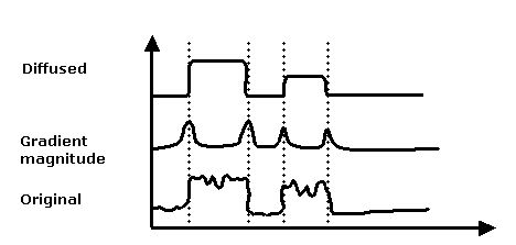
Figure 1 illustrates the relationship between anisotropic diffusion and gradient magnitude. In the figure, the original signal is noisy but two major peaks are still visible. Applying the diffusion process to the original signal and using the gradient magnitude to attenuate the diffusion process at places where the edge is strong produces a signal in which the overall signal-to-noise ratio has improved. |
 |
Background
The following is the anisotropic diffusion equation:
Equation 1
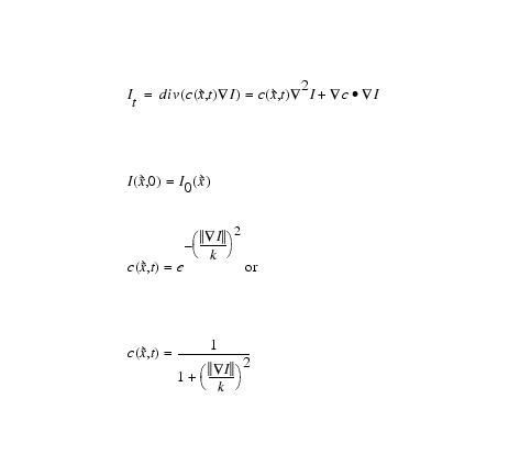 |
where ![]() is the variable conductance term. Typically, a function of the gradient magnitude
is the variable conductance term. Typically, a function of the gradient magnitude ![]() , if
, if ![]() is a constant, then
is a constant, then ![]() which is the isotropic heat diffusion equation (Gaussian blurring).
which is the isotropic heat diffusion equation (Gaussian blurring).
In simple terms, the image I at some time t is given by the diffusion of the image where conductance term limits the diffusion process. This program uses a conductance term calculated by dividing a constant (k) divided by the square root of the sum of the squares of the normalized first order derivatives of the Gaussian function as an approximate gradient function. Figure 2 shows the result of applying this technique. The image on the left is a CT image before processing. The image on the right of it was diffused. Note the image was diffused within object boundary but to a much lesser amount near the boundaries of the objects.
Image types
You can apply this algorithm just to gray-scale images.
 |
Special notes
Refer to the section on Filters (Spatial): Nonlinear Noise Reduction.
References
Refer to the following references for more information:
P. Perona and J. Malik. "Scale-Space and Edge Detection Using Anisotropic Diffusion," IEEE 'Trans. Pattern Analysis and Machine Intelligence, 12(7):629-639, July 1990.
Bart M. Ter Romeney, ed. Geometry-Driven Diffusion in Computer Vision. (Dordrecht, The Netherlands: Kluwer Academic Publishers, 1994).
Applying the Anisotropic Diffusion algorithm
To run this algorithm, complete the following steps:
- Open an image.
- Perform, as an option, any image processing, such as improving the contrast, eliminating noise, etc., on the image.
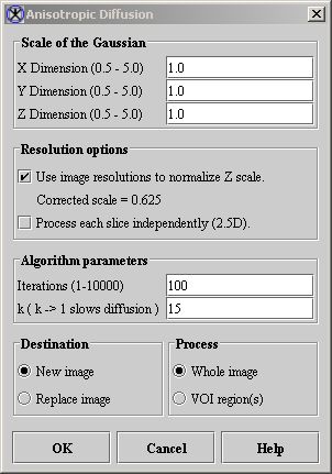
- Select Algorithms > Filters (spatial) > Anisotropic Diffusion. The Anisotropic Diffusion dialog box (Figure 3) opens.
- Complete the information in the dialog box.
|
|
Note: Diffusing an image is a lengthy process. Give some consideration to the values you type into the Iterations and k boxes. The higher the number of iterations slows processing speed as does a small k value. |
- Click OK. The algorithm begins to run.
- A pop-up window appears with the status. The following message appears
- "Diffusing image."
- When the algorithm finishes running, the pop-up window closes.
- Depending on whether you selected New image or Replace image, the results appear in a new window or replace the image to which the algorithm was applied.
|
X dimension
(0.5 - 5.0)* |
Indicates the standard deviation (SD) of Gaussian in the X direction.
|
 |
|
Y dimension
(0.5 - 5.0)* |
Indicates the SD of Gaussian in the Y direction.
| |
|
Z dimension
(0.5 - 5.0)* |
Indicates the SD of Gaussian in the Z direction.
| |
|
Use image resolutions to normalize Z scale
|
Normalizes the Gaussian to compensate for the difference if the voxel resolution is less between slices than the voxel resolution in-plane. This option is selected by default.
| |
|
Process each slice independently (2.5D)
|
Blurs each slice of the dataset independently.
| |
|
Iterations
(1-1000) |
Specifies the number of times the process is run.
| |
|
k (k > 1 slows diffusion)
|
Specifies the constant used to control the blurring rate. A small value slows the diffusion process (especially across edges) per iteration. A large value speeds the diffusion process but also allows for diffusion (blurring across edges); it also makes this function act similar to Gaussian blurring. See equation above.
| |
|
New image
|
Shows the results of the algorithm in a new image window.
| |
|
Replace image
|
Replaces the current active image with the results of the algorithm.
| |
|
Whole image
|
Applies the algorithm to the whole image.
| |
|
VOI regions
|
Applies the algorithm to the volumes (regions) delineated by the VOIs.
| |
|
OK
|
Applies the algorithm according to the specifications in this dialog box.
| |
|
Cancel
|
Disregards any changes you made in this dialog box and closes the dialog box.
| |
|
Help
|
Displays online help for this dialog box.
| |
|
*An SD greater than 1 attenuates small scale edges typically caused by noise, but reduces edge accuracy.
| ||