Shading Correction: Inhomogeneity N3 Correction

This preprocessing algorithm corrects for shading artifacts often seen in MRI. The heart of the algorithm is an iterative approach that estimates both a multiplicative bias field and a distribution of true tissue intensities. Referred to as nonparametric intensity nonuniformity normalization (N3), this method makes no assumptions about the kind of anatomy present in a scan and is robust, accurate, and fully automatic.

Background

A common difficulty with tissue intensity model based methods is the determination of the model. The modeling assumption in the N3 algorithm is that of a field model: the assumption that nonuniformity blurs the histogram of the data in a way that it can be identified, quantified, and removed. This nonuniformity blurring distribution is referred to as the blurring kernel F. The following equation is the basis of the N3 method:

Equation 1

Where at location x, v is the measured signal, u is the true signal emitted by the tissue, f is an unknown smoothly varying bias field, and n is white Gaussian noise assumed to be independent of u. As can be seen, the unknown smoothly varying bias field f multiplies the true signal u, thereby corrupting it. Then the additive noise n is added, resulting in the output measured signal v. To compensate for the intensity nonuniformity, the first task is to estimate its distribution, or f.

Then taking the log of all parameters, we are left with ^u = log(u) and ^f=log(f), both of which we assume to be independent or uncorrected random variables of probability densities U, V, and F. Then substituting these variables back into equation 1 and converting the equation of distributions into one of probability densities, the distribution of their sum turns into the following convolution, see equation 2

Equation 2

Equation 2 models the nonuniformity distribution F viewed as blurring the intensity distribution U.

Now the model of intensity nonuniformity used here is that of a multiplicative field corrupting the measured intensities. However, viewing the model from a signal processing perspective, one sees that there is a much more specific consequence, a reduction of only high-frequency components of U. Thus, the approach used in the N3 algorithm to correct for nonuniformity turns into an optimization problem, which goal is to maximize the frequency contents of U.

How the N3 method works

We begin with only a measured distorted signal, or image, which we call v. For computational purposes, we do not deal with simple v, but instead, with log^v and the histogram distribution of the log, and use ^v to denote V. The same representations are used for the true signal, u, and the distortion signal, f.

The model assumed here is that of a multiplicative biasing field that multiplies the true signal to distort it, thereby creating a signal with induced field inhomogeneity. So, just as a multiplication takes place to corrupt the field, a division should undo the corruption. Now carrying this idea over to the frequency domain where all of the computations take place, multiplications turn into convolutions and divisions turn into deconvolutions.

To begin with, all one has is v. Users provide a value for the kernel full-width, half maximum (FWHM) of f. Then, the iteration takes place as this estimate of f is later used to compute U and then U input back into the algorithm to create another mapping, another f, and hence another U. The process then repeats until convergence. The result is an estimated true value of U.

Mapping from v to f

The approach adopted for finding U depends largely on the mapping from v to f. The idea is to propose a distribution of U by sharpening the distribution V and then estimating the corresponding smooth field log(f), which produces a distribution U close to the one proposed. However, rather than searching through the space of all distributions U, one can take advantage of the simple form of the distribution F. Suppose the distributions of F is Gaussian. Then one need only search the space of all distributions U corresponding to Gaussian distributed F having zero mean and given variance. In this way the space of all distributions U is collapsed into a single dimension, the width of the F distribution. Thus, concludes the mapping N3 creates from v to f.

Estimating u throughout an entire volume:

Equation 3

Estimating u (voxel by voxel):

Equation 4

Algorithm flow chart

This algorithm performs the process shown in the flow chart in Figure 1. What was previously described was just the basic algorithm idea. The equations behind the steps in the process are shown in an enlarged section of the flow chart in Figure 2.

The algorithm does the following:

1. Identifies the foreground. In this step, the algorithm thresholds the background.
2. Resamples to working resolution. Use the input working resolution "subsampling factor."
3. Logs transform intensities.
4. Obtains the expectation of the real signal. Given a measured signal, the algorithm obtains the expectation of the real signal by performing a voxel by voxel difference between the logs of signal and estimate bias field.
5. Obtains an initial estimate of distribution U. The algorithm estimates distribution U, where U is a sharpened distribution of V. The sharpening is done using input parameters FWHM and Z. Given a distribution F and the measured distribution of intensities V, the distribution U can be estimated using a deconvolution filter as follows:
   Equation 5
   

   
   

   Equation 6

   
   and

   

   where

   F* denotes complex conjugate
   '~F is the fourier transform of F
   Z is a constant term to limit the magnitude of ~G
   This estimation of U is then used to estimate the corresponding field.
   

6. Computes the expectation of real signal-The algorithm computes the expectation of the real signal given measured signal (both logged). Full volume computation done using distributions U and Gaussian blurring kernel F (whose FWHM parameter is given by users). A basic mapping from v to f. This is the iterative portion, which is shown the main loop in Figure 1.
7. Obtains a new field estimate-The difference between the measured signal and the newly computed expectation of the real signal given the measured signal (all variables logged). Equation 7
   

   
   

8. Smooths the bias field estimate-Using the B-spline technique with the parameter d field distance input provided by users.
   Equation 8
   

   
   

9. Terminates iterations-The algorithm then checks for the convergence of field estimates. If the subsequent field estimate ratio becomes smaller than the end tolerance parameter input by users, the iterations are terminated. If not, a new F is used in step 2, and the iteration repeats step 4 through step 9.
   Equation 9
   

   
   where r'n is the ratio between subsequent field estimates at the n-th location, s -denotes standard deviation, and m denotes mean. Typically after 10 iterations, e drops below 0.001.

10. Completes the final steps-Given the measured signal, obtain the expectation of the real signal by calculating a voxel by voxel difference between logs of signal and an estimate of the bias field. Once iteration is complete, exponential transform intensities V and F, extrapolate field to volume, resample data back to original solution. Then divide v by f. The result is u.
    Equation 10
    

    
    

    Figure 1. Flow chart describing the N3 method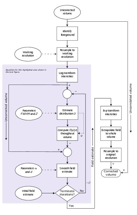

    
    

    Figure 2. The N3 method showing the equations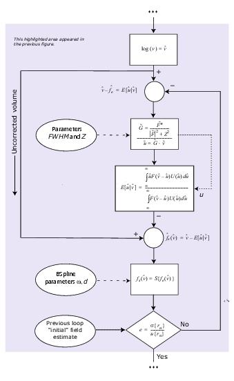

    Figure 3. The effect of N3 on an image: (A) original image and (B) image after N3 correction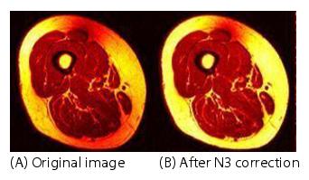

    
    

    Figure 3 shows an original image A and the image B produced from using the best N3 paratmeters:

    • Treshold = 100
    • Maximum iterations = 100
    • End tolerance = 0.0001
    • Field distance = 33.33
    • Subsampling factor = 2
    • Kernel FWHM = 0.8
    • Wiener = 0.01

    Figure 4 shows an original image and the effect of different parameters used in the Inhomogeneity N3 Correction algorithm on the image.

    Figure 4. The effects of different settings for the Inhomogeneity N3 algorithm on an image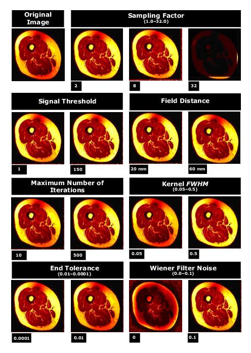

    Image Types

    You should apply this algorithm only to 2D and 3D MRI images.

    References

    Refer to the following sources for more information about the N3 algorithm.

    Sled, John G., Alex P. Zijdenbos, and Alan C. Evans. "A Nonparametric Method for Automatic Correction of Intensity Nonuniformity in MRI Data." IEEE Transactions on Medical Imaging, 17(February 1998):87-97.
    Sled, John G. "A Non-Parametric Method for Automatic Correction of Intensity Non-uniformity in MRI Data." Masters thesis, Department of Biomedical Engineering, McGill University, May 1997.