MIPAV DTI pipeline interface
Main article: DTI Pipeline.
The MIPAV DTI pipeline allows the user to upload and process diffusion weighted images (DWIs), and then it computes voxel-wise diffusion tensors (DT) for the further |analysis of diffusion tensor imaging (DTI) data. It determines an anatomical correspondence between DTI and structural MRI images (T2) of the same sample. As an output, the pipeline computes maps of diffusion eigenvalues and eigenvectors and creates visualization of fibers tracts going through a specific VOIs.
The MIPAV DTI Pipeline interface contains 6 tabs:
- In the Import Data tab the user uploads DW and T2 image (optional), and the gradient information (optional). Or, MIPAV reads the gradient information from the image header. The Phillips Gradient Creator will then calculate the gradient table based on provided information.
- In the Pre-processing tab, the user can specify the parameters required for rigidly registering B0 to T2, and then DWI to the rigidly registered B0, and also parameters for motion correction and eddy current distortion correction.
- In the EPI Distortion Correction tab, the user enters parameters needed to calculate deformation vector fields for rigidly aligned B0 and T2 from the Pre-processing step.
- In the Tensor Estimation tab, the user uploads the mask image, selects the tensor estimation algorithm and specifies the output options.
- In the Tensor Statistics tab the user can upload the tensor image and specifies which kind of images (e.g. ADC, color map, Eigen value, Eigen vector, FA, RA, and Volume Ratio.) he/she would like to have as an output.
- In the Visualization tab, the user can upload images needed for a 3D visualization of fiber bundle tracts in the brain's white matter using the information. The user can then save fiber tracts information as .vtk and .dat files.
Import Data tab
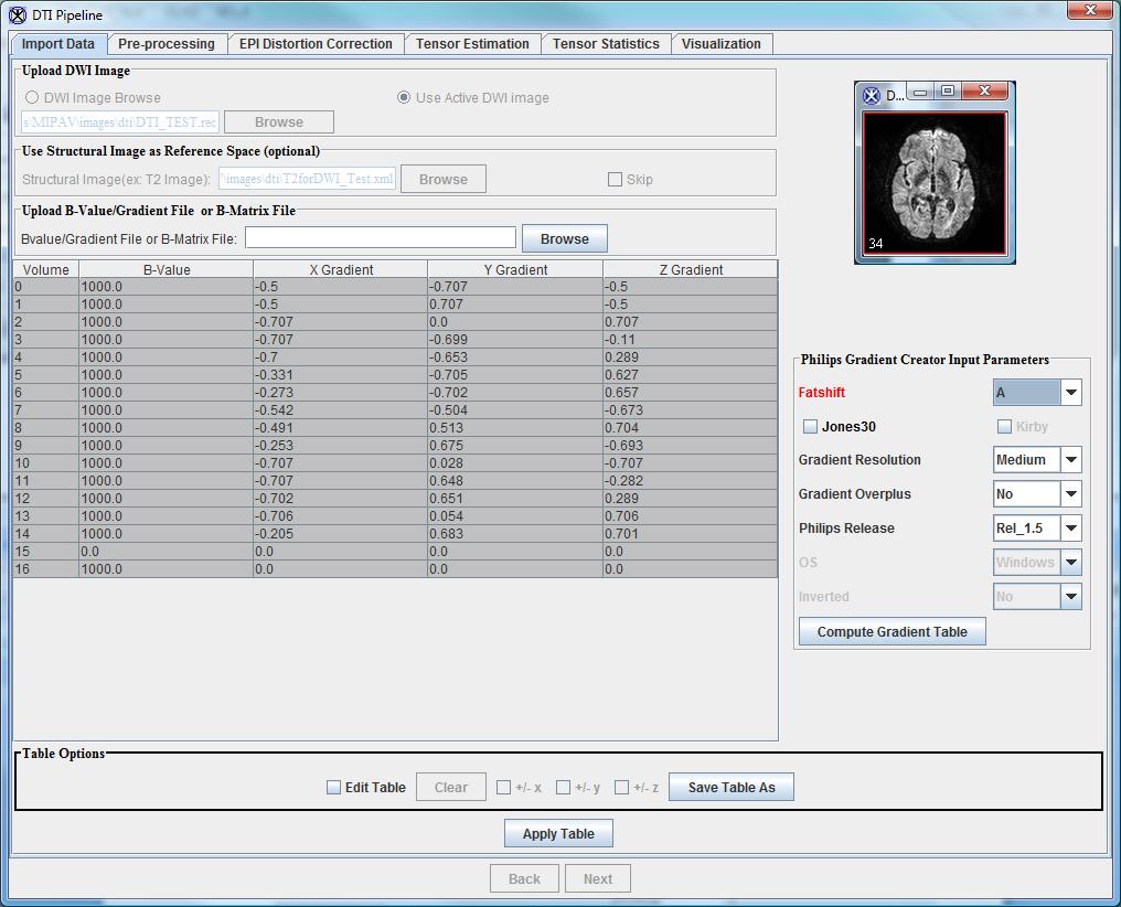
This panel is for uploading DW and T2 images, calculating gradients,uploading B-matrix information, and creating the B-matrix/Gradient table. DTI Pipeline reads raw data in all MIPAV supported formats and DICOM files.
Upload DWI Image box
DWI Image Browse – check this option if you would like to upload your image of interest from your computer.
Use Active DWI Image – check this option to use an active image, which is already opened in MIPAV.
Note: in MIPAV, an active image is the one that has a red frame.
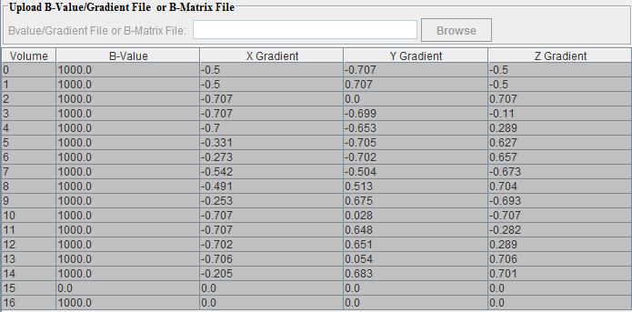
Uploading B-Value/Gradient File or B-Matrix file
This option allows a user to manually upload B-Value/Gradient File or B-Matrix file. See also: Table Options.
Gradient vector file is a 3D set of coordinates representing the direction (on the form of a vector) along which a magnetic gradient has been applied. Each DTI pulse sequence has a set of gradient vectors associated with it. This set is required for subsequent analysis.
B-value is a scaling factor used to describe the attenuating effect of the MR signal on the different gradients. A diffusion gradient can be represented as a 3D vector, where the direction of vector is in the direction of diffusion and its length is proportional to the gradient strength. The gradient strength, or more often used diffusion weighting parameter term, is expressed in terms of the B-value parameter, which is proportional to the product of the square of the gradient strength (q) and the diffusion time interval (b ~ q2 • Δt). Read more: MRI TIP database.
Philips Gradient Creator

The Philips Gradient Creator computes the correct gradient table which is necessary to calculate diffusion tensors. The table lists gradient vectors that describe the diffusion weighting directions, which are later used for analysis and computing diffusion tensor. The Gradient Creator works with data acquired by Philips MRI scanners. Note: the Philips Gradient Creator options would not appear for images from other scanners.
It uses the source code from DTI_gradient_table_creator created by Jonathan Farrell, Ph.D.
The code that computes the gradient table based on minimal user input. The list of input parameters is show below, see Gradient Creator input parameters. You can also refer to Jonathan Farrell's web site for additional information.
The specifications of the gradient table created for the image taken on Philips MRI scanner(s) are determined by:
- The 3 coordinate frames defined on the MR scanner: world, anatomical, and image coordinate system. For more information, refer to Slicer WIKI.
- The rules on how imaging options (including slice orientation, slice angulation, phase encoding direction, etc.) impact the gradient directions.
- The scanner software release.
- Any motion correction, if performed.
Slice angulation
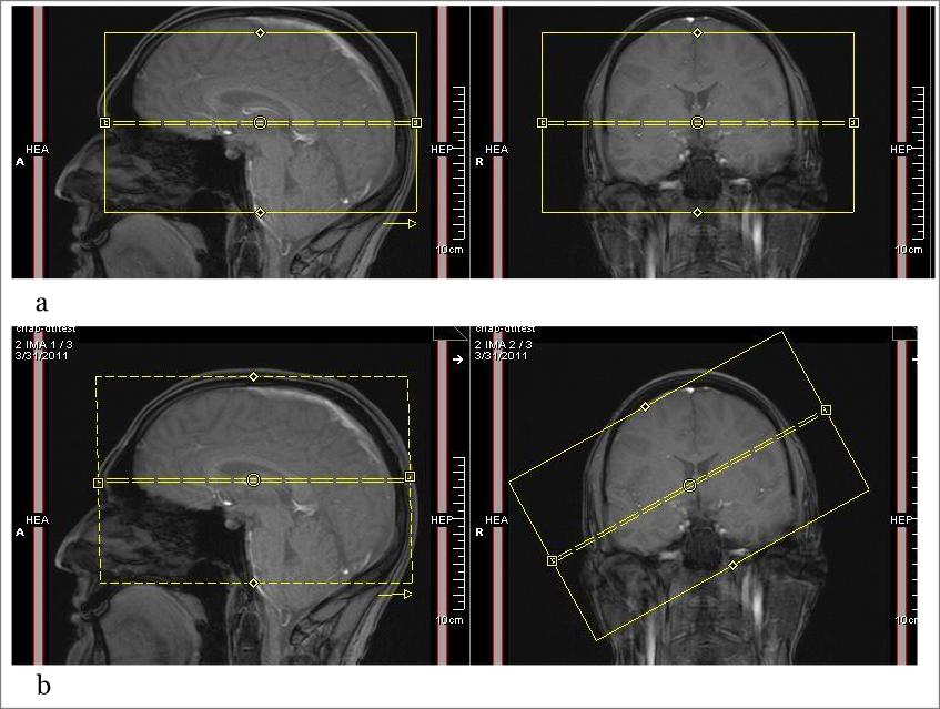
In diffusion tensor imaging (see [1]), tensors are constructed by collecting a series of direction-sensitive diffusion images. MRI scanners save these directions along with the images and later they are used to reconstruct the diffusion properties of the images.
Depending on the scanner, the vectors are recorded with reference either to the scanner bore, or to the imaging grid. This should not a problem if the images are acquired precisely orthogonal to the scanner bore, because in that case the image and the scanner share the same frame of reference.
Problems can arise in oblique acquisitions when the image plane is not aligned with the scanner bore. In this situation, it is important that the gradient vectors used in the imaging software are in the same frame of reference as the image. This requires conversion or re-ordering, otherwise we will get angulation errors.
Note: these angulation errors have little influence on the DTI parameters, which are invariant to tensor rotation - ADC, MD and FA. However, they do affect calculation of the eigenvectors of the tensor.
The Gradient or B-Matrix table
In the Gradient or B-Matrix table, if gradients are displayed, the 2nd column contains B values, while X Gradient, Y Gradient and Z gradient columns contain the diffusion gradients applied along the x, y, and z axis - Gx, Gy, and Gz correspondingly.
If B-matrix is displayed, 6 b-values are displayed per volume including bxx, byy, bxy, bxz, byz, and bzz.
Gradient creator input parameters
| Gradient Creator Parameters | Options | Philips PAR/REC Version |
|---|---|---|
| Fatshift | R: Right L: Left A: Anterior P: Posterior H: Head F: Feet |
V3 & V4 V4.1 & V4.2 |
| Jones30 or Kirby | Specify which MRI scanner was used to acquire DW images. This option works for KKI scanners only. | V3 & V4 V4.1 & V4.2 |
| Gradient Resolution | Low: used for 8 DWI volumes Medium: used for 17 DWI volumes High: used for 34 DWI volumes |
V3 & V4 V4.1 & V4.2 |
| Gradient Overplus | Yes No |
V3 & V4 V4.1 & V4.2 |
| Philips Release | Rel_1.5 Rel_1.7 Rel_2.0 Rel_2.1 Rel_2.5 Rel_11.x |
V3 & V4 V4.1 & V4.2 |
| Patient Position | Head First Feet First |
V3 & V4 |
| Patient Orientation | SP: Supine PR: Prone RD: Right Decubitus LD: Left Decubitus |
V3 & V4 |
| Fold Over | AP: Anterior-Posterior RL: Right-Left FH: Head-Feet/ Superior-Inferior |
V3 & V4 |
| OS (Operating System) | Windows VMS |
V3 & V4 V4.1 & V4.2 (for KKI scanners only) |
| Inverted | No Yes |
V3 & V4 V4.1 & V4.2 (for KKI scanners only) |
Compute Gradient Table - use this button to compute the gradient table based on data you entered into Gradient Input Parameters.
Error messages
"Gradient Table Creator Image dimensions 17 are not consistent with gradient table choice - exacted 8 dimensions" or a similar message means that Gradient Resolution (e.g. Low, Medium, High) did not correspond to the volume number of the image you uploaded to the pipeline. In this example, the “Gradient Resolution” was set to “Low” which corresponds to 8 volumes/dimensions, while the image had 17 volumes. In order to calculate the gradient table, we needed to change the “Gradient Resolution” parameter to “Medium".
"Gradient Table Creator R: is not consistent with Anterior-Posterior fold over" or a similar message means that the Fold Over option selected does not match the image specification. In order to solve that problem, select the correct fold over option.
Table Options
The Table Options box allows the user to directly edit the values in the the Gradient table and to save the updated table. To edit the table, press the Edit button. To save the table, press Save Table As. The table could be save in various formats, including Plain text (.txt), FSL, dtistudio and MIPAV standard format.
Applying the gradient table
When a user entered all parameters needed for the Philips Gradient Table Creator, the Apply Table button becomes available to apply the changes and save the DTI parameters in the file header (if the file is saved in MIPAV XML format).
Specials notes
For more information regarding the importing DW images, refer to Jonathan Farrell's web site - http://godzilla.kennedykrieger.org/~jfarrell/software_web.htm.
- If your DTI data was acquired on a Philips MR Scanner with new software (release version 1.5, 1.7, 2.0 or 2.1), the PAR file version may be V4.1. You can verify this by looking at the top right hand corner of the file for the following tag: Research image export tool V4.1. The other known versions are V3 or V4.
- The V4.1 PAR files list the diffusion weighting directions, however, these directions are provided not in the image space (see Slice angulation). Specifically, in the case the Gradient Overplus option is set to YES, the directions need to be rotated and corrected for slice angulation. This is automatically done by the Gradient Table creator.
- The Gradient Table Creator does not read gradient directions from some PAR file because this information is not available for all PAR files (V3 or V4). It uses the directions documented in the Philips source code instead.
Import Data tab output files
The gradient and B-matrix table files are the output files from the Import Data tab. They can be saved in a user specified folder in different formats, e.g. dtistudio, FSL, or MIPAV XML format.
Note: Siemens Mosaic 3D DICOM files if used as an input, would be saved as 4D volumes based on corresponding B-matrix volumes.
Pre-processing tab
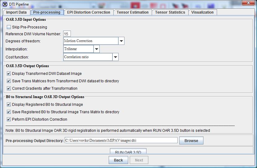
In this tab, the user can specify parameters for running OAR 3D (or OAR 3.5D) algorithm that will perform the rigid registration of B0 to T2 and then DWI to rigidly aligned B0. OAR 3.5D is used to correct the spatial mis-registration of DWI volumes originating from both - subject motion and eddy current-induced distortions. The user has a choice to run OAR 3D or OAR 3.5D. For more information about both algorithms, refer to the OAR documentation.
Note: if a used doesn't have a T2 image, the registration could still be performed based on the B0 volume, but the user choice would be limited by OAR 3.5 D algorithm only.
OAR 3.5D input options
- Skip Pre-Processing - check this box if you would like to skip the entire step.
- Reference DWI volume number - usually MIPAV can figure out the reference volume number (this is B0 volume), but in case MIPAV missed it, a user can enter the reference volume number in the space provided.
- Degrees of freedom - in MIPAV, this parameter provides the number of independent pieces of information that are used to calculate the transformation. The user has an option to select either Motion Correction, or Motion Correction + Eddy current. See also Affine Transformations.
- Interpolation - in this box, a user can select the interpolation method to use. The list includes following interpolations: Trilinear, B-spline 3rd order, B-spline 4th order, Cubic Lagrangian, Quintic Lagrangian, Heptic Lagrangian, and Windowed sinc.
- Cost Function - in this box, a user can specify a cost function that would be used in the registration. The list of available cost functions is as follows: Correlation ratio, Least squares, Normalized cross-correlation, Normalized mutual information.
OAR 3.5D output options
- Display Transformed DWI dataset image - check this box if you would like to view the transformed DWI dataset.
- Save trans matrices from transformed DWI dataset to directory - check this box, if you would like to save transformation matrices to an chosen Output directory.
- Correct gradients after transformation - check this box, if you would like MIPAV to correct the initial gradient information. See Gradient Creator.
B0 to structural image OAR 3D output options
- Display registered B0 to structural image: - if this box is checked, the result image would be displayed in a separate window.
- Save registered B0 to structural image trans matrix to directory: - if this box is checked, the transformation matrix would be saved in the user specified directory.
- RUN OAR 3.5D - press this button to run the algorithm.
- Output dir: - here a user can specify the directory that would be used to save output and intermediate files, such as transformation matrices and registered B0 volumes.
OAR output files
The output files are as follows:
- the B0 volume rigidly registered to the structural (T2) image
- the transformation matrix from B0 rigidly registered to the structural image
- the re-sampled structural (T2) image from the OAR algorithm
EPI Distortion Correction tab
Clinical diffusion MR studies are mostly based on single-shot echo-planar imaging (EPI) acquisitions. This method is very sensitive to static magnetic field inhomogeneities and artifacts, which appear due to imperfection of the gradient waveforms, and eddy currents during the long readout time. These issues are primarily responsible for creating nonlinear geometric distortion along the phase-encoding direction. Artifacts often appear at air-tissue border and also in the images of the ventral portions of the frontal and temporal lobes. They become even more severe with increasing magnetic field. The mis-registration among a set of DWI volumes due to geometric distortions leads in turn to spatial inaccuracies in the derivation of the diffusion tensor, ADC, and FA since they are typically computed on a pixel-by-pixel basis combining all diffusion-weighting directions.
To correct geometric distortions due to B0 inhomogeneities, MIPAV uses the special image registration technique, where the distorted EPI image is registered to a corresponding anatomically correct MR image with an intensity based least-squares similarity metric and the VABRA modeled deformation field to improve the sensitivity in areas of low EPI signal.
References
- Chen B., Guo H., Song A.W., Correction for Direction-Dependent Distortions in Diffusion Tensor Imaging Using Matched Magnetic Field Maps, Brain Imaging and Analysis Center, Duke University, Media: DTIdistortionCorrection.pdf
- Rohde G.K., Student Member, IEEE, Aldroubi A., and Dawant B.M., Senior Member, IEEE, The Adaptive Bases Algorithm for Intensity-Based Nonrigid Image Registration, IEEE TRANSACTIONS ON MEDICAL IMAGING, VOL. 22, NO. 11, NOVEMBER 2003, Media: VabraRegistration2003.pdf
- Wu M., Chang L.-C, Walker L., Lemaitre H., Barnett A.S, Marenco S., and Pierpaoli C., Comparison of EPI Distortion Correction Methods in Diffusion Tensor MRI Using a Novel Framework, 2008, Media: EpiDistortionCorrection.pdf
Computing the deformation field
All fields except "Compute deformation field" are populated automatically with data from the Pre-processing tab. However, the user has the option to manually upload previously saved files.
- Reference DWI volume number - MIPAV can determine the reference volume number (this is B0 volume). However, if the usedr would like to enter a different number, he/she can do it in the space provided. Also if the DWI has multiple B0 volumes, the number of B0 of interest could be also entered by the user.
- Resampled T2 image - this field refers to the resampled T2 image from the Pre-processing tab. In case the field did not get populated automatically, the user has an option to upload the image using the Browse button.
- Registered DWI image - this field refers to the registered DWI volume from the Pre-processing tab. In case the field did not get populated automatically, the user has an option to upload the image using the Browse button.
- Output dir: - by default, this field refers to the same Output directory which was indicated in the Pre-processing tab. The user has an option to indicate/change the path to the Output directory using the Browse button.
- Display deformation field - if this box is checked, MIPAV will display deformation field after calculation.
- Display B0 registered to T2 - if this box is checked, MIPAV will display B0 registered to T2 calculation.
- Compute deformation field - press this button to start computation. MIPAV uses the VABRA non-linear registration method to compute deformation field. Note that depending on your computer capabilities, this operation migh take a considerable time.
VABRA note: VABRA stands for Vectorized Adaptive Bases Registration Algorithm - a deformable registration algorithm, which is an intensity-based nonrigid registration algorithm. As an output, it returns a registered image and the applied deformation field. For more information, refer to the VABRA web site.
MIPAV API note: for API information regarding MIPAV VABRA algorithm, refer to VABRA API.
Computing EPI distortion correction
After computing the deformation field, MIPAV creates the following files:
- Deformation field file (in XML format)
- B0 to T2 transformation matrix (.mtx)
- 4D transformation matrix (.mtx)
They make the input for the EPI distortion correction algorithm.
- Deformation field - this field is populated automatically from the Pre-processing step. However, the user could also manually upload the file using the Browse button.
- B0 to T2 transformation matrix - this field is also populated automatically from the Pre-processing step. However, the user could also manually upload the file using the Browse button.
- 4D transformation matrix - this field is also populated automatically from the Pre-processing step. However, the user could also manually upload the file using the Browse button.
- Display EPI-distortion corrected image - by default, this box is checked.
- Compute EPI-distortion correction - press this button to start computation.
Tensor Estimation tab
This module estimates the diffusion tensor model from a given DWI Volume. The result is a tensor volume that can be used to compute different anisotropy measurements, for example Fractional Anisotropy, and also perform fiber tractography.
- Mask Image - is an approximated mask of the white matter that can be used to filter out the background. The mask image is optional, however, it should be uploaded by the user when using CAMINO Non-linear and/or CAMINO Restore algorithm.
Tensor estimation algorithms
The following algorithms (available via the DTI algorithm drop-down menu) are used in the pipeline:
Weighed, noise-reduction - this is the default method used in MIPAV DTI pipeline. It is based on the book by S. Mori, "Introduction to Diffusion Tensor Imaging".
LLMSE - is based on CATNAP pipeline.
The following 3 methods have been ported from Camino. Camino is a fully-featured toolkit for Diffusion MR processing and reconstruction. For more information, refer to: Cook et al (2006).
CAMINO: Linear - this algorithm uses unweighted linear least-squares to fit the diffusion tensor to the log measurements. The algorithm is based on the method explained in the paper by Basser P.J., Mattielo J., and Lebihan D. (1994).
CAMINO: Non-linear - this method provides more accurate noise modelling than Linear fitting. The algorithm is based on the method explained in papers by Jones and Basser (2004) and Alexander and Barker (2005).
CAMINO: Restore - this algorithm fits the diffusion tensor robustly in the presence of outliers, for more information refer to the CAMINO Tutorial. The algorithm is based on the method explained in the paper by Chang, Jones and Pierpaoli (2005).
CAMINO: Weighed linear - this algorithm uses a weighted linear fit, as originally proposed by Jones and Basser (2004).
References
- Alexander D.C. and Barker G.J., "Optimal imaging parameters for fibre-orientation estimation in diffusion MRI", NeuroImage, 27, 357-367, 2005,Abstract.
- Basser P.J., Mattielo J., and Lebihan D., "Estimation of the effective self-diffusion tensor from the NMR spin echo, Journal of Magnetic Resonance", 103, 247-54, 1994, [[Media:Basser1994.pdf], Abstract
- Chang L-C, Jones D.K. and Pierpaoli C., "RESTORE: Robust estimation of tensors by outlier rejection, Magnetic Resonance in Medicine", 53(5), 1088-1095, 2005, PDF
- Cook P. A., Bai Y., Nedjati-Gilani S., Seunarine K. K., Hall M. G., Parker G. J., Alexander D. C., "Camino: Open-Source Diffusion-MRI Reconstruction and Processing", 14th Scientific Meeting of the International Society for Magnetic Resonance in Medicine, Seattle, WA, USA, p. 2759, May 2006, Abstract
- Jones D.K. and Basser P.J., "Squashing peanuts and smashing pumpkins: How noise distorts diffusion-weighted MR data", Magnetic Resonance in Medicine, 52(5), 979-993, 2004, PDF
- Mori S., "Introduction to Diffusion Tensor Imaging", ISBN-10: 0444528288 | ISBN-13: 978-0444528285, ScienceDirect, Media:SMori2008.pdf
Output Options
The following output options available for all tensor estimation algorithms:
- Save Tensor image - when this box checked, MIPAV saves the tensor image in the Output directory.
- Display Tensor image - when this box checked, MIPAV displays the tensor image.
The following output options available only for tensor estimation algorithms based on CAMINO code:
- Save Exit Code image - when this box checked, MIPAV saves the tensor image in the Output directory.
- Display Exit Code image - when this box checked, MIPAV displays the exit code image. The exit code is set 0 in brain voxels and -1 in background voxels.
- Save Intensity image - when this box checked, MIPAV saves the tensor image in the Output directory.
- Display Intensity image - when this box checked, MIPAV displays the intensity image.
- Output directory - the directory that is used to save output and intermediate files.
Tensor Statistics tab
- Tensor image - MIPAV populated this field automatically with a path to the tensor image created in the Tensor Estimation tab. However, a user has an option to upload the file using the Browse button.
Output options
The user could use the following check boxes to specify what kind of images they want to create/display.
| Output options | |||||
|---|---|---|---|---|---|
| Create ADC image | Display ADC image | ||||
| Create Color image | Display Color image | ||||
| Create Eigen Value image | Display Eigen Value image | ||||
| Create Eigen Vector image | Display Eigen Vector image | ||||
| Create RA image | Display RA image | ||||
| Create FA image | Display FA image | ||||
| Create Trace image | Display Trace image | ||||
| Create VR image | Display VR image | ||||
- Output dir: - in this field, the user could specify the directory that would be used for output files.
Visualization tab
Please refer to the GPU computing page in order to learn how to enable MIPAV GPU Volume Renderer required for DTI visualization.
This is the final step of the MIPAV DTI pipeline. It allows the user to specify Volumes of Interests (VOIs) and to display fibers tracts going through a specific VOI. The users can also seed individual fiber tracts based on mouse clicks. In visualization, local diffusivity of the white matter is represented by glyphs including ellipses cylinders, lines, tubes, and arrows.
In this panel, the user is asked to upload the following images created in the Tensor Statistics panel: tensor image, color image, EVector image, FA image EValue image, and T2 image, which is the original T2 image. Note that in the most cases, MIPAV will upload these images automatically.
After uploading all images, press the Load button to start visualization.