Visualizing Images: Displaying images using the default view:Changing image brightness and contrast using LUTs
From MIPAV
Changing image brightness and contrast using LUTs
Generally, computer systems have brightness display values written in the display hardware. These values are known as the physical color map; they are hard coded in your monitor. When you open an image, the image file contains data that indicates the intensity of each voxel in the image. These data are passed to the physical color map and displayed on the monitor. Additionally, MIPAV provides a logical color map, which allows you to remap the original intensities to other intensities. Although technically the term look-up table (LUT) can be used for the physical and logical color maps, in this guide look-up table refers to the logical color map only. You can apply predefined, pseudo color or inverse LUTs, or you can manually manipulate the transfer function used to map the image data to the LUT. The LUT then translates the remapped values so that they can be interpreted by the physical color map and displayed on your monitor.
To adjust the look-up table using the Quick LUT
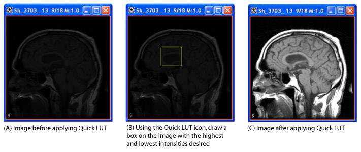
To adjust the LUT, you open the Look-up Table window to modify the LUT's values and transfer function. However, you can use the Quick LUT icon to modify the LUT without opening the Look-up Table window. Quick LUT allows you to easily choose the highest and lowest values for the intensity levels in a user- defined area.
To do this, complete the following steps:
1 Open an image.
2 Click  (Quick LUT) in the MIPAV window.
3 Move the cursor to the image window and draw a box around an area that has the highest and lowest intensities you want the image to display. These values are used to remap the image data to the LUT. The net effect is increased contrast in the area of interest (Figure 14).
Figure 118. An image before and after applying Quick LUT
|
Â
Â
Â
{| align="center"
|
|
|}
To generate a histogram and look-up table
A histogram is a graphic representation of the intensity level distribution in an image or VOI region. It displays the number of voxels at each intensity level. The histogram and LUT appear in the Look-up Table window.
To generate a histogram, and view the LUT, complete the following steps:
1 Open an image. The image appears in an image window.
2 Create a VOI on the image (optional step).
3 Do either of the following:
Click Look-up Table.
Select LUT > Histogram -LUT.
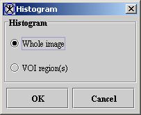
If the image contains a VOI, the Histogram window appears (Figure 15). Go to the next step.
Figure 119. Histogram dialog box
|
{| align="center"
|
|
|}
If there are no VOIs on the image, the Look-up Table window (Figure 16) appears.
4 Choose one of the following:
Whole image-To generate a histogram for the whole image
VOI region(s)-To generate a histogram for the VOI region of the image
5 Click OK. A progress message appears briefly. After a few moments, the Look-up Table window appears (Figure 16).
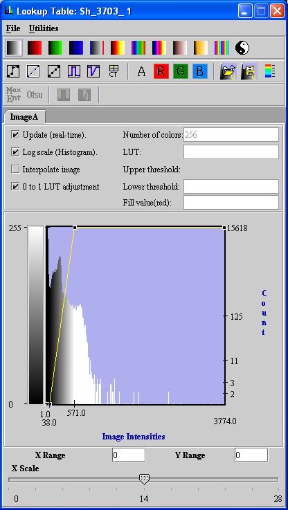
Figure 120. Look-up Table windowÂ
|
File
|
Open LUT-Opens a previously saved LUT file. LUT files have a .LUT extension. Save LUT-Saves the LUT displayed in this window in a LUT file. Open Transfer Functions-Opens a previously saved transfer function. Transfer function files have a .FUN extension. Save Transfer Functions-Saves the transfer function displayed in this window to a file. Close LUT-Closes the LUT window.
|
{| align="center"
|
|
Â
Â
Â
Â
Â
Â
Â
Â
Â
Â
Â
Â
|-
| rowspan="2" colspan="1" |
Utilities
|
Change number of colors-Allows you to change the number of colors displayed in the image.
Valid values are 2 to 256.
|-
| rowspan="1" colspan="2" |
CT function-Allows you to select a preset LUT that is appropriate for the image content. Values are abdomen, head, lung, mediastinum, spine, and vertebrae.
Invert LUT-Creates a negative of the image.
Reset histogram and LUT A-Returns image A to its original values.
Reset histogram and LUT B-Returns image B to its original values. This command is only available if two images are open.
|-
|
LUT toolbar
| rowspan="1" colspan="2" |
Provides tools that allow you to manipulate the displayed image. Refer to Figure 19.
|-
|
Update (real-time)
| rowspan="1" colspan="2" |
Changes the image as you make changes to the LUT, which allows you to see the effect of your changes immediately on the image.
|-
|
Log scale (histogram)
| rowspan="1" colspan="2" |
Displays the image's histogram count in log scale along the Y axis.
|-
|
Interpolate image
| rowspan="1" colspan="2" |
Displays image using interpolation, which reduces pixilated image to appear more smooth.
Caution: Depending on the memory resources of your workstation, interpolation can be very lengthy.
|-
|
Number of colors
| rowspan="1" colspan="2" |
Allows you to change the number of colors displayed in the image.
|-
|
LUT
| rowspan="1" colspan="2" |
Displays the image intensities.
|}
The Look-up Table window consists of three sections: a menu bar, a toolbar, and one or more pages containing histograms. A tab appears for each image that is opened in the image window. For example, if only one image is in the image window, then only the Image A tab appears. If you generated the histogram for an image window that contains two images, a tab for Image A and a tab for Image B appear. Each of these tabbed pages contain a histogram for the applicable image. If you generated the histogram for a VOI, the window does not display a tab and only the applicable icons and buttons in the toolbar appear.
The toolbar allows you to manipulate the displayed image. You can apply pseudocolor LUTs, adjust the image contrast with the transfer function, and apply preset window and level settings for CT slices. You can also edit the red, blue, green, and alpha channels of a LUT.
look-up table (LUT)-Indicates the intensity of each voxel in the image and, in MIPAV, allows you to remap the original intensities to other intensities.
transfer function-Reflects the relationship between the original image intensity values and how they are mapped into the LUT. The line in the LUT represents the transfer function.
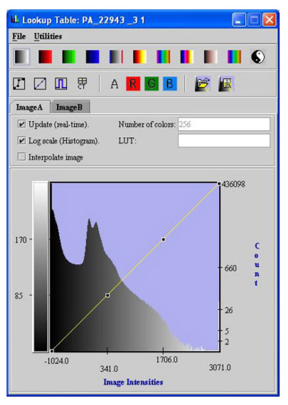
Note: You can generate a histogram for two image datasets that are loaded together. In this case, the Look-up Table window (Figure 17) shows two tabs-one for Image A and one for Image B.
Figure 121. Look-up Table window showing Image A and B histograms
|
{| align="center"
|
|
|}
To update images in real time
When you modify the LUT, be sure to select the Update (real time) check box. The image in the image window is then updated in real time.
To change the number of intensities displayed in the LUT
You can change the number of intensities displayed in the LUT. To do this, do the following:
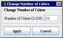
1 Select Utilities > Change Number of Colors in the LUT window. The Change Number of Colors dialog box opens.
Figure 122. Change Number of Colors dialog box
|
{| align="center"
|
|
|}
2 Type the number of colors you want in the Number of colors box. You can specify any whole number between 2 and 256.
3 Select Apply to apply the changes.
Notice that the Number of colors box in the LUT window now displays the number you specified and the histogram changes to display the new colors.
4 Click Close or Cancel to close the dialog box.
Applying predefined LUTs to images
You can use MIPAV's predefined LUTs to apply pseudocolor, create a negative of the image, and apply preset CT window and level settings to an image.
To apply pseudocolor LUTs to images
As you examine an image, you may need to observe small changes in intensity values or identify the same intensity values in different portions of an image. This can be difficult if the image is rendered in grayscale because the human eye can only see about 100 shades of gray. However, because varied colors are often easier to distinguish, MIPAV allows you to use various pseudocolor maps to elucidate objects of interest. Thus, MIPAV provides a variety of pseudocolor LUTs. If you apply a pseudocolor LUT, the grayscale intensity values are remapped to color intensity values. Note that the original image data is not changed; only the displayed image file (hence the term pseudocolor).
Figure 123. LUT toolbar
|
{| align="center"
|

|
|}
To apply a pseudocolor LUT, click one of the following icons:
 Red LUT
 Green LUT
 Blue LUT
 Gray blue/red LUT
 Hot metal LUT
 Spectrum LUT
 Cool hot LUT
 Striped LUT
 Invert LUT
The grayscale intensity values in the image dataset are remapped to color intensity values.
To invert intensities
To invert the intensities so that a negative of the dataset appears, click  , the Invert LUT icon. The Invert LUT icon is in both the Look-up Table window (Figure 16 on page 26) and the MIPAV window. Figure 19 on page 30 shows the location of this icon in the Look-up Table window.
To apply CT level presets to images
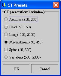
There are six CT window and level presets: abdomen, head, lung, mediastinum, spine, and vertebrae. To apply a preset level to the image, complete the following steps:
1 Click  , the CT Preset icon, in the LUT window. The CT Presets dialog box appears (Figure 20).
Figure 124. CT Presets dialog box
|
{| align="center"
|
|
|}
2 Select the desired CT preset. As you select the CT preset option, the colors in the image's histogram or LUT change, and, if you chose to update images in real time, the image changes.
3 Click OK to save the change.
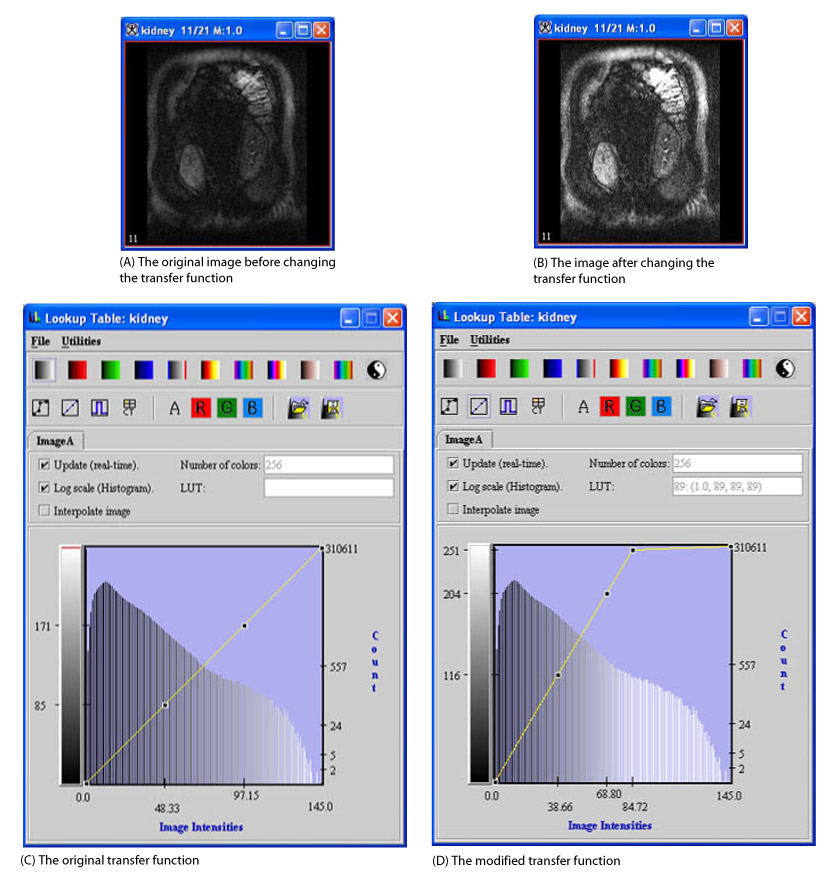
Adjusting contrast using the transfer function
The transfer function reflects the relationship between the original image intensity values and how they are mapped into the LUT. An example of how adjusting the transfer function affects the display of an image appears in Figure 16. In this example, the top image is generated by applying the linear transfer function (slope = 1) to produce display values that are evenly distributed over the range of the LUT (see [MIPAV_VisualizationTools.html#1995063 Figure 125]A). This results, in this case, in a low-contrast image (see [MIPAV_VisualizationTools.html#1995063 Figure 125]B). The contrast of the image can be improved by adjusting the transfer function in a manner shown in [MIPAV_VisualizationTools.html#1995063 Figure 125]A (e.g., changing a low-contrast image into a high-contrast image). The image scalar values between -175 and 275 are remapped as a function of the modified transfer function and distributed across the full LUT range. The values above 275 are remapped to white and the values below -175 are remapped to black. The effect can be readily seen in [MIPAV_VisualizationTools.html#1995063 Figure 125]B.
To modify transfer functions
1 Open an image. The image appears in the default image window.
2 Click  , the Displays Look-up Table (LUT) icon. The Look-up Table dialog box opens.
3 Click the transfer function. A new node may appear.
4 Drag the node to the new location.
You can also adjust the transfer function for the alpha, red, green, and blue channels in an image.
Example: You might want to use these icons to highlight certain intensities in a particular color.
To do this, click the appropriate one of the following icons:
 , the Edit Alpha icon
 , the Edit Red icon
 , the Edit Green icon
 , the Edit Blue icon
When you click on one of these icons, the transfer function for that channel appears on the histogram and a node appears on that transfer function. Drag the node to the desired position. To adjust another channel, you must click on the icon and drag the node to the appropriate position.
Figure 125. An image before and after modifying the transfer function
|
{| align="center"
|
|
Â
|}
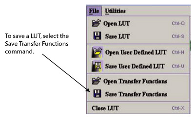
To save transfer functions
To save a transfer function to a file, complete the following steps:
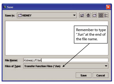
1 In the Look-up Table dialog box, select File > Save Transfer Functions ([MIPAV_VisualizationTools.html#1171663 Figure 126]) or press Ctrl S. The Save dialog box ([MIPAV_VisualizationTools.html#1171682 Figure 127]) appears.
Figure 126. Open and Save commands in the File menu
|
{| align="center"
|
|
|}
2 Type a name to the transfer function in the File Name box. Be sure to add the .fun extension to the file name.
Figure 127. Save dialog box
|
{| align="center"
|
|
|}
3 Click Save. The program saves the transfer function under the name you specified.
To apply previously saved transfer functions
To open a transfer function file and apply it to an image, complete the following steps:
1 Select File > Open Transfer Functions in the Look-up Table window. The Open dialog box appears.
2 Select the desired file. LUT files have a .fun extension.
3 Click Open. The program applies the transfer functions file to the current image.
To save LUTs for later use
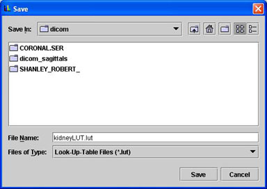
1 Select File > Save LUT in the Look-up Table window, or press Ctrl S. The Save dialog box ([MIPAV_VisualizationTools.html#1171713 Figure 128]) appears.
Figure 128. Save dialog box
|
{| align="center"
|
|
|}
2 Type a name for the LUT in the File Name box. Be sure to add the .lut extension to the file name.
3 Click Save. The program saves the LUT under the name you specified.
To open and apply previously saved LUTs to images
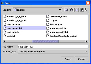
1 Select File > Open LUT in the Look-up Table window, or press Ctrl O. The Open dialog box (Figure 25) appears.
2 Select the desired file. LUT files have a .lut extension.
3 Click Open. The program applies the LUT settings from the LUT file you specified to the current image file.
Figure 129. Open dialog box
|
{| align="center"
|
|
|}
To open, save, and apply frequently used LUTs
For a LUT that you defined and expect to use frequently, MIPAV provides a simple method for saving, opening, and applying it without needing to use the commands on the File menu. You use two icons on the toolbar in the Look-up Table window:
 , the Save User-Defined LUT icon, allows you to save the LUT.
 , the Open User-Defined LUT icon, provides a very quick way of opening and applying the user-defined LUT
{| align="left" | File:MIPAV VisualizationTools59.gif |}
Recommendation: Because these icons only apply to one user-defined LUT, it is recommended that you select the LUT that is used most frequently.
To reset original LUTs to images
Click  , the Grayscale icon in the Look-up Table window (refer to Figure 16 and Figure 19). Alternatively, you can click
  , the Reset LUT icon, in the MIPAV window.
To adjust the threshold
1 Open an image. The image appears in the default image window.
2 Click , the Displays Look-up Table (LUT) icon. The Look-up Table dialog box opens.
3 Click  , the Dual threshold function icon. The Threshold icon becomes active and the transfer function of the histogram changes.
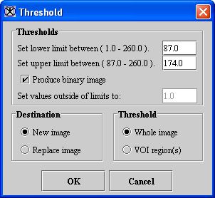
4 Select Algorithms > Threshold. The Threshold dialog box (Figure 26) opens.
Figure 130. Threshold dialog boxÂ
|
Set lower limits between (1.0-3774.0)
|
Threshold limit for the lowest image intensities.
|
{| align="center"
|
|
|-
|
Set threshold between (1258.3334-3774.0)
|
Threshold limit for the highest image intensities.
|-
|
Produce binary image
|
Produces a binary image (Boolean).
|-
|
Set values outside of limits to
|
Specifies the intensity value to assign to values outside the threshold limits.
|-
|
New image
|
Shows the results of the algorithm in a new image window
|-
|
Replace image
| rowspan="1" colspan="2" |
Replaces the current active image with the results of the algorithm.
|-
|
Whole image
| rowspan="1" colspan="2" |
Applies the algorithm to the whole image.
|-
|
VOI regions
| rowspan="1" colspan="2" |
Applies the algorithm to the volumes (regions) delineated by the VOIs.
|-
|
OK
| rowspan="1" colspan="2" |
Applies the changes you made in this dialog box and closes the dialog box.
|-
|
Cancel
| rowspan="1" colspan="2" |
Disregards any changes you made in this dialog box, closes the dialog box, and does not change the threshold.
|-
|
Help
| rowspan="1" colspan="2" |
Displays online help for this dialog box.
|}
5 Complete the dialog box.
Note: You can choose to generate a binary image (Boolean) by selecting the Produce binary Image check box. Alternatively, you can clear the binary option and enter a threshold value. If you still want to generate a Boolean image, select the check box again. Note that, if you generate a Boolean image, MIPAV does not allow you to reapply the threshold or to generate either a histogram or LUT for a Boolean image.
6 Click OK to apply the threshold.
Visualizing Images: Displaying images using the animate view


