File list
From MIPAV
This special page shows all uploaded files.
| Name | Thumbnail | Size | User | Description | Versions | |
|---|---|---|---|---|---|---|
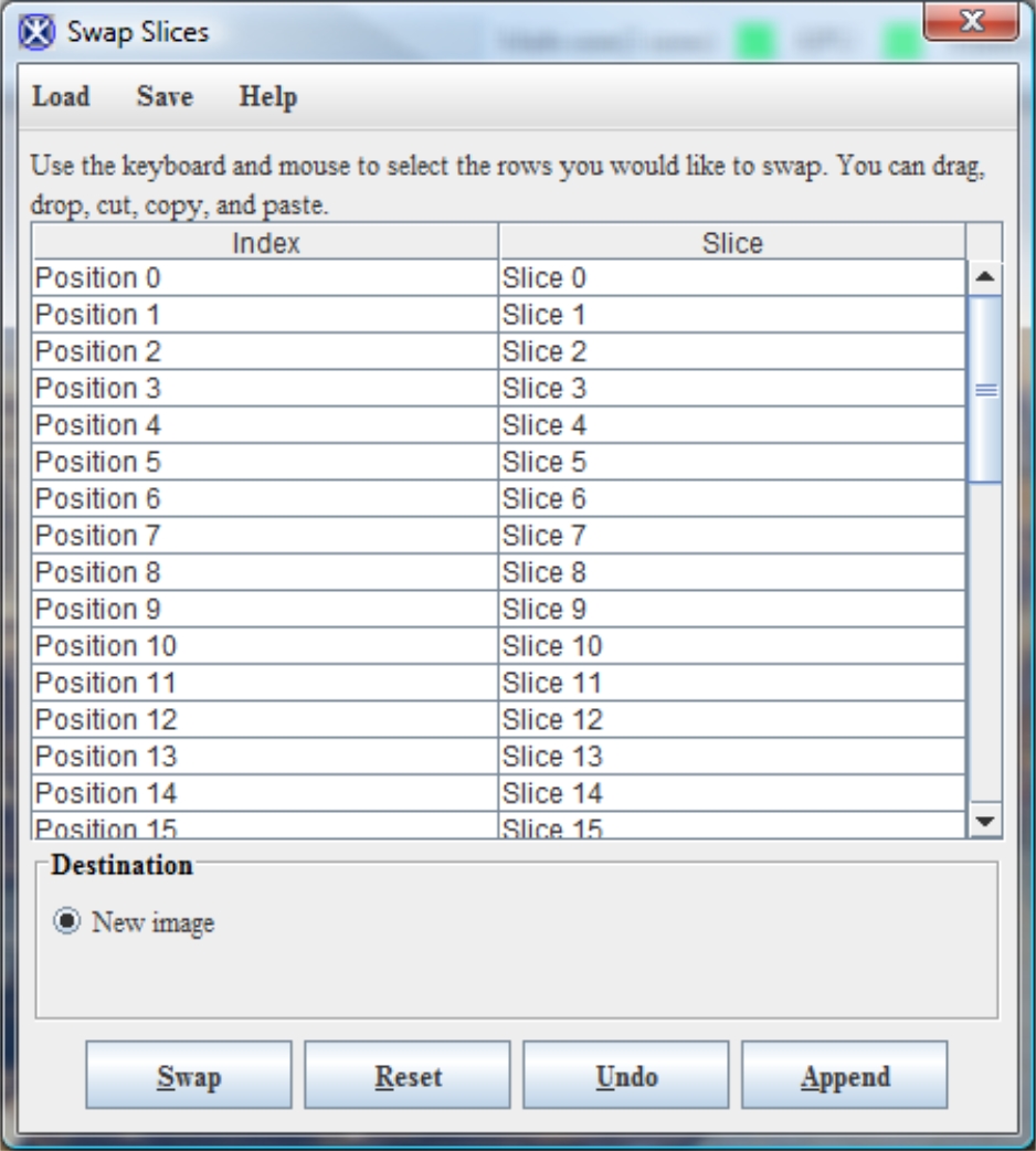
| 13:24, 7 September 2012 | SwapSLicesDialogBox.jpg (file) |  |
347 KB | Olga Vovk | 3 | |
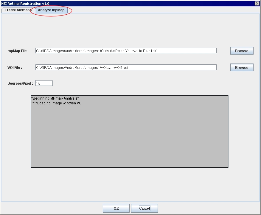
| 12:56, 28 August 2012 | AnalyzepMapFiletab.jpg (file) |  |
104 KB | Olga Vovk | NEI Retinal Registration: Analyze mpMap tab | 1 |
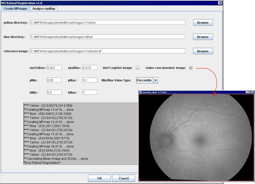
| 12:50, 28 August 2012 | CreateMPmapTab.jpg (file) |  |
264 KB | Olga Vovk | NEI Retinal Registration: Create MP maps tab | 1 |
| 12:47, 28 August 2012 | OutputDirectories.jpg (file) |  |
116 KB | Olga Vovk | NEI Retinal Registration: Figure - Output Directories: The plug in's input and output catalogs: given the Blue and Yellow as the input catalogs, the plug in created Output1, BlueReg1 and YellowReg1 catalogs after the first run and Output2, BlueReg2 and Ye | 1 |
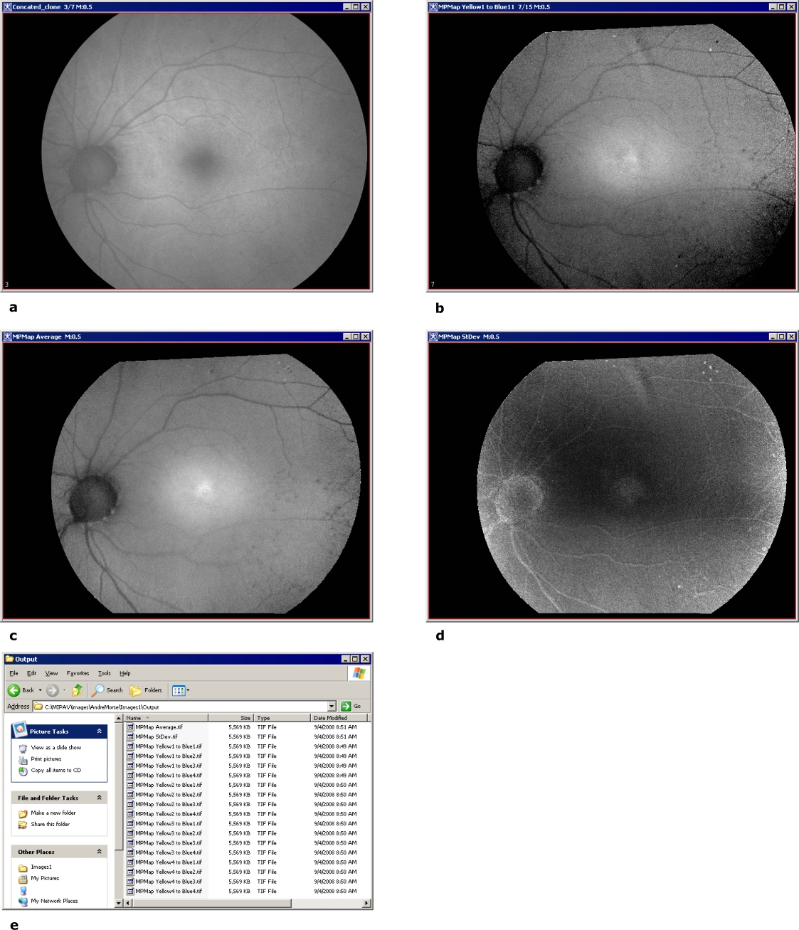
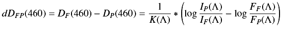
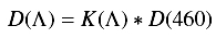
| 12:39, 28 August 2012 | Examples.jpg (file) |  |
632 KB | Olga Vovk | NEI Retinal Registration plug-in: Figure: (a) - the registered image, (b) - the MP map Yellow1 to Blue1 image, (c) - the MP map average image, (d) - the MP map standard deviation image, and (e) the Output directory | 1 |
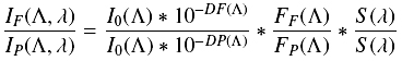
| 18:36, 27 August 2012 | NEIPlugInEQ4.jpg (file) | 27 KB | Olga Vovk | NEI retinal registration - equation4 | 1 | |
| 18:31, 27 August 2012 | NEIPlugInEQ3.jpg (file) | 15 KB | Olga Vovk | NEI Retinal registration equation 3 | 1 | |
| 18:13, 27 August 2012 | NEIPlugInEQ2.jpg (file) | 26 KB | Olga Vovk | NEI retinal registration plug-in, equation 2 | 1 | |
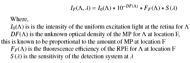
| 18:05, 27 August 2012 | NEIPlugInEQ1.jpg (file) |  |
80 KB | Olga Vovk | NEI Retinal Registration: In equation 1, absorbers other than the MP and fluorophores other than RPE lipofuscin are neglected to simplify the process. Typically, contributions from rhodopsin absorption will confound these measurements. In typical Fundus c | 1 |
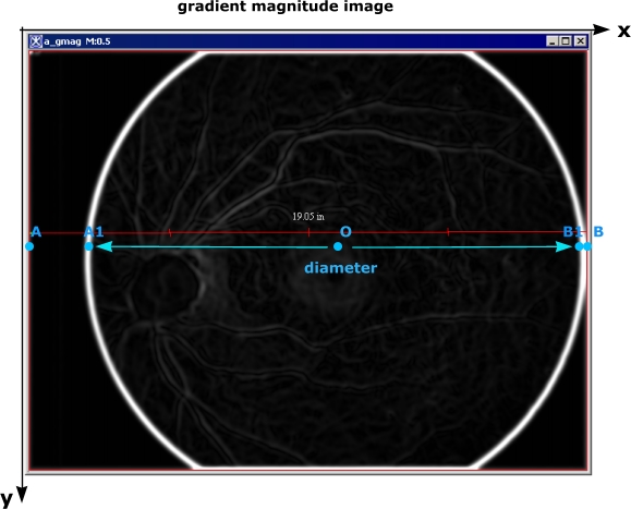
| 17:02, 27 August 2012 | RemovingBorder.jpg (file) |  |
96 KB | Olga Vovk | NEI Retinal registration plug -in: Removing the black border from the GM image: A1 and B1 are the far left and right non border pixels, O is the center pixel | 1 |
| 19:39, 20 August 2012 | SarahShenPosterAugust2012.pdf (file) | 911 KB | Olga Vovk | NIH’s Summer Research Program Poster Day 2012 August 9, 2012 | 1 | |
| 13:38, 20 August 2012 | CircleToRectangle1a.jpg (file) |  |
590 KB | Olga Vovk | Transformation: Conformal mapping: Circle to Rectangle - The user inputs 2 point VOIs. The first point is located at the center of the circle. The second point can be any point located on the actual circle | 1 |
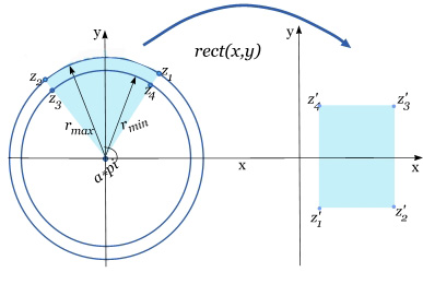
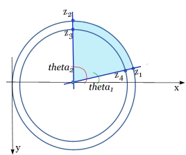
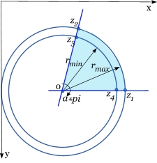
| 18:52, 17 August 2012 | CircularSectorToRectangleMapped.jpg (file) |  |
37 KB | Olga Vovk | Transform Conformal Mapping: The region inside a circular sector is mapped to a rectangle: z1 is the upper right point on rmax, z2 is the upper left point on rmax, z3 is the lower left point on rmin, and z4 is the lower right point on rmin | 1 |
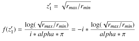
| 16:58, 17 August 2012 | Equation11.jpg (file) |  |
28 KB | Olga Vovk | 1 | |
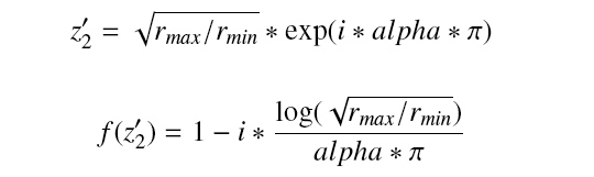
| 16:58, 17 August 2012 | Equation10.jpg (file) |  |
31 KB | Olga Vovk | 1 | |
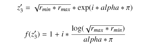
| 16:58, 17 August 2012 | Equation9.jpg (file) |  |
29 KB | Olga Vovk | 1 | |
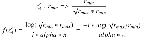
| 16:57, 17 August 2012 | Equation8.jpg (file) |  |
33 KB | Olga Vovk | 1 | |
| 15:48, 17 August 2012 | CircularSectorToRectangleAngle.jpg (file) |  |
26 KB | Olga Vovk | Transform Conformal Mapping : Calculating the angle of the circular segment | 2 |
| 15:45, 17 August 2012 | ConfMappingCircleCenter.jpg (file) |  |
27 KB | Olga Vovk | Transform Conformal mapping: Calculating the center of the circle to which the circular segment belongs | 1 |
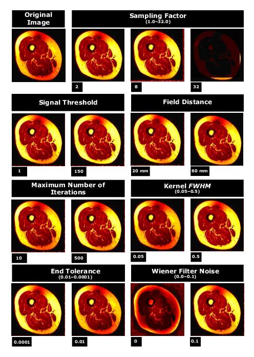
| 13:43, 13 August 2012 | N3Effects5.jpg (file) |  |
77 KB | Olga Vovk | Shadig Correction N3 inhomo . correction - Figure 4. The effects of different settings for the Inhomogeneity N3 algorithm on an image | 2 |
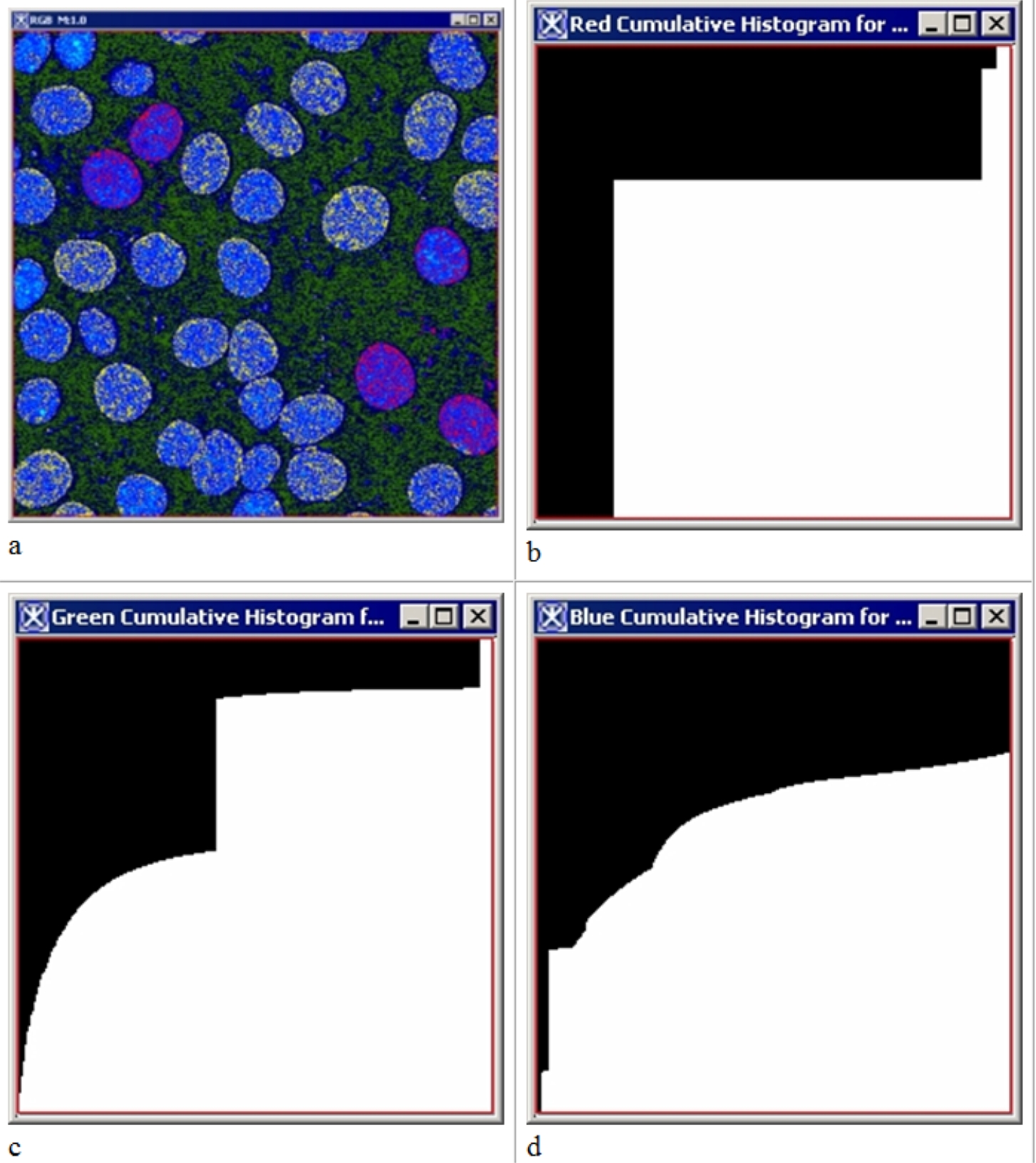
| 15:04, 7 August 2012 | Fig14CumulativeHistogram.jpg (file) |  |
588 KB | Olga Vovk | A 2D RGB image and its cumulative histograms | 1 |
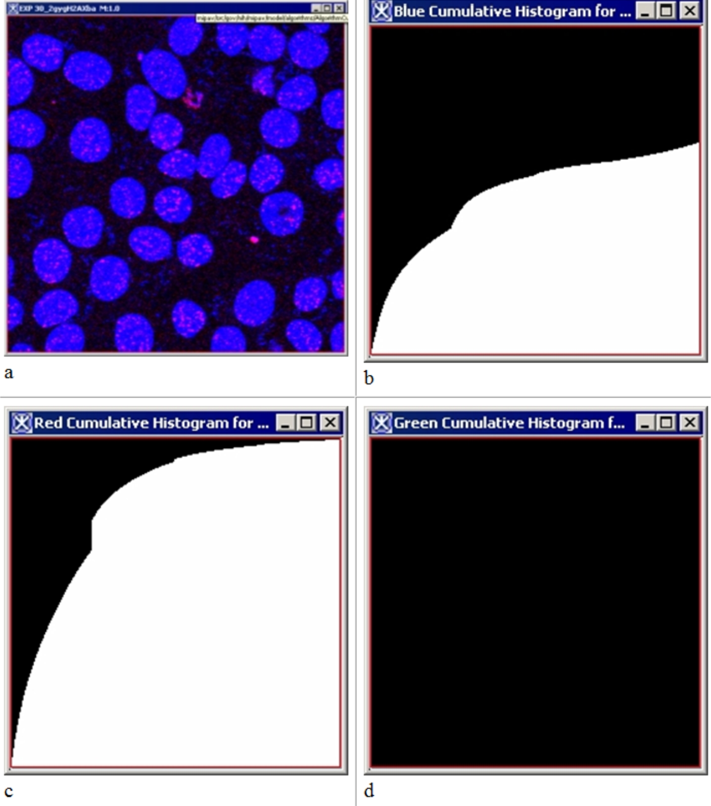
| 15:01, 7 August 2012 | Fig13CumulativeHistogram.jpg (file) |  |
491 KB | Olga Vovk | A 2D RGB image and its cumulative histograms for each channel (red -c, green-d and blue-b). | 1 |
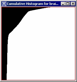
| 14:55, 7 August 2012 | CumulHistogramBrain2CH.jpg (file) |  |
21 KB | Olga Vovk | A 3D grayscale image (a) and its cumulative histogram (b). | 2 |
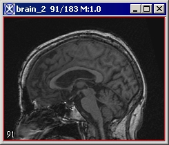
| 14:54, 7 August 2012 | CumulHistogramBrain2.jpg (file) |  |
40 KB | Olga Vovk | A 3D grayscale image (a) and its cumulative histogram (b). | 2 |
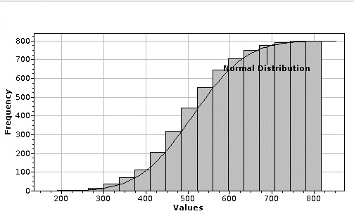
| 14:49, 7 August 2012 | CumulativeHistogramSample.jpg (file) |  |
53 KB | Olga Vovk | A sample cumulative histogram | 2 |
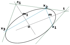
| 13:55, 7 August 2012 | HoughEllipseGeometry.jpg (file) |  |
25 KB | Olga Vovk | Hough Transform: Calculating a center of an ellipse: x1, x2, x3 - three ellipse points; (t, x1), (t, x2) and (t, x3) the tangents of the points x1, x2 and x3 correspondingly; m is the midpoint of (x1, x2), m1 is the midpoint of (x2, x3); o is the center o | 1 |
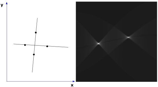
| 13:11, 7 August 2012 | TwoLinesHoughTransform.jpg (file) | 17 KB | Olga Vovk | Hough Transform: The two bright spots are the Hough parameters of the two lines. From these spots' positions, r and theta parameters for two lines in the input image can be determined | 2 | |
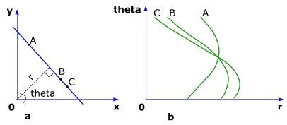
| 13:06, 7 August 2012 | ParametricLineHough.jpg (file) |  |
24 KB | Olga Vovk | Parametric Hough transform: (a) a straight line in the original coordinates described in terms of the length of a normal from the origin to the line - r and orientation theta; (b) the Hough plane where points A, B, and C are transformed into three sinusoi | 2 |
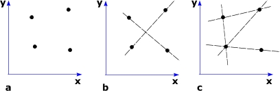
| 13:04, 7 August 2012 | LinearHough.jpg (file) |  |
17 KB | Olga Vovk | A set of image points (a), and how they can be fit into various line segments - (b) and (c) | 2 |
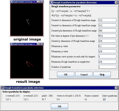
| 19:29, 6 August 2012 | HoughParabolaDB.jpg (file) |  |
108 KB | Olga Vovk | Running the Hough Transform for Parabola Detection algorithm. Note that the detected parabola appears in red | 2 |
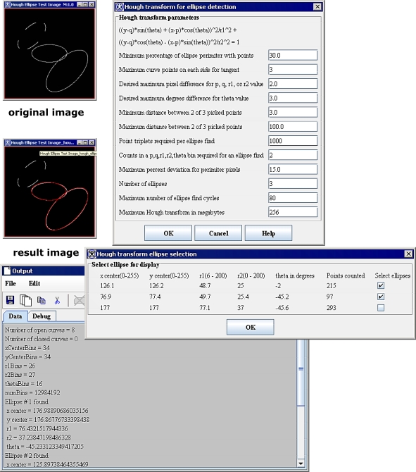
| 19:24, 6 August 2012 | HoughEllipsesDialogBoxes1.jpg (file) |  |
182 KB | Olga Vovk | Running the Hough Transform for Ellipse Detection algorithm. Note that isolated ellipses checked for display appear in red | 2 |
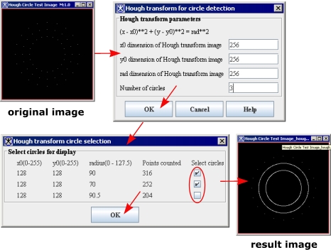
| 19:19, 6 August 2012 | HoughCirclesDialogBoxes.jpg (file) |  |
86 KB | Olga Vovk | Running the Hough Transform for Circle Detection algorithm. Note that only two of three isolated circles are shown in the result image, because only two were checked in the Hough Transform Circle Selection dialog box | 2 |
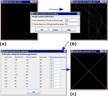
| 19:17, 6 August 2012 | LinearHoughTransformAlgorithm.jpg (file) | 67 KB | Olga Vovk | Running the Hough Transform for Line Filling algorithm | 2 | |
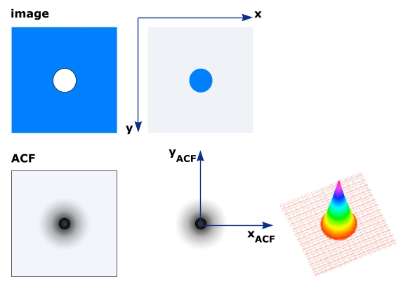
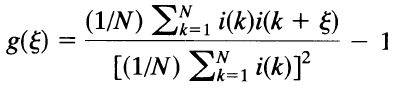
| 17:05, 6 August 2012 | AutocorrScheme.jpg (file) |  |
50 KB | Olga Vovk | AutoCorrelation Function: Visualization of ACF | 2 |
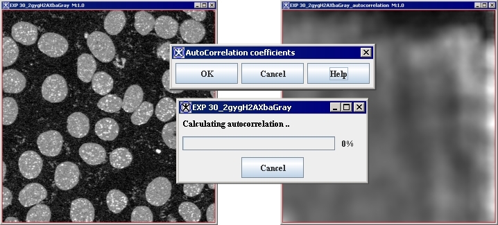
| 16:47, 6 August 2012 | AutocorrDialog.jpg (file) |  |
155 KB | Olga Vovk | Autocorrelation: Calculating autocorrelation for 2D grayscale image | 2 |
| 16:18, 6 August 2012 | AutoCovar12D.jpg (file) | 35 KB | Olga Vovk | Auto covariance coeff: For a discrete set of data this becomes | 1 | |
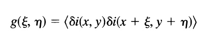
| 16:17, 6 August 2012 | AutoCovar11D.jpg (file) | 20 KB | Olga Vovk | Autocovariance coeff: If the random intensity variable, i, is a function of two independent variables, x and y, then, it is possible to define a corresponding two-dimensional auto-covariance function | 1 | |
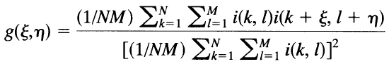
| 16:16, 6 August 2012 | AutoCovar10D.jpg (file) | 27 KB | Olga Vovk | When the data consist of a set of N discrete points, the averaging is performed as sums, then in spatial domain the 1D auto-covariance function is calculated by | 1 | |
| 13:45, 6 August 2012 | WaterShedDialogHelp.jpg (file) |  |
52 KB | Olga Vovk | The Watershed dialog box | 2 |
| 13:15, 6 August 2012 | WatershedIll4Small.jpg (file) |  |
21 KB | Olga Vovk | Watershed algorithm: (c) - the result image | 2 |
| 13:13, 6 August 2012 | WatershedIll3Small.jpg (file) |  |
123 KB | Olga Vovk | Watershed algorithm: (c) the result segmented image | 3 |
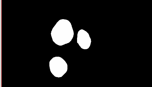
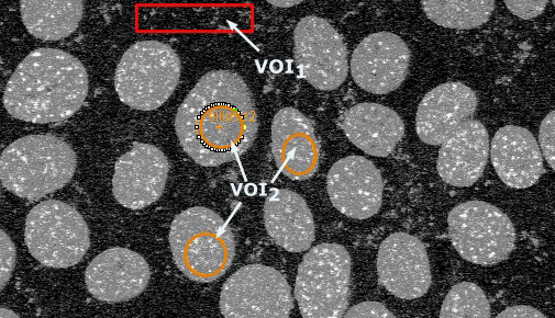
| 13:12, 6 August 2012 | WatershedIll2Small.jpg (file) |  |
117 KB | Olga Vovk | Watershed algorithm: (a) - the original image with two VOIs: the VOI1 highlights the image background and VOI2 is a group of three VOI delineated inside the objects we wish to segment | 2 |
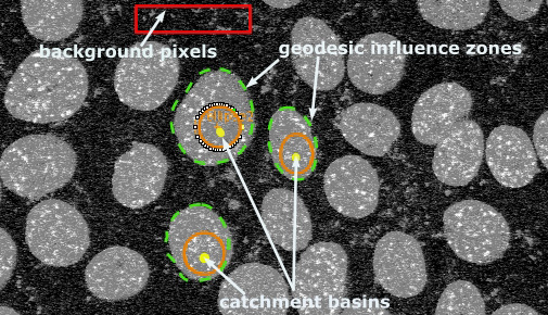
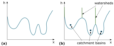
| 13:05, 6 August 2012 | Watershed1D.jpg (file) |  |
32 KB | Olga Vovk | Figure 1. 1D example of watershed segmentation: (a) grey level profile of the image data, (b) watershed segmentation | 2 |
| 16:45, 31 July 2012 | DialogBoxFRETEfficiencyColor.jpg (file) |  |
101 KB | Olga Vovk | FRET Efficiency dialog box | 1 |
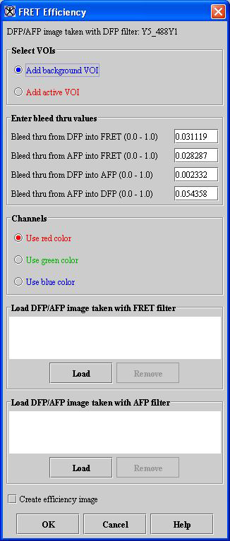
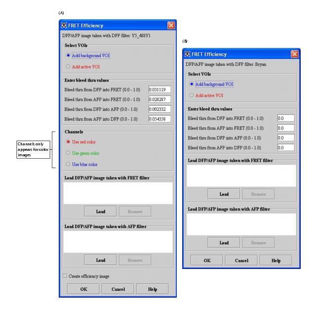
| 16:37, 31 July 2012 | DialogBoxFRETEfficiency.jpg (file) |  |
50 KB | Olga Vovk | FRET Efficiency dialog box (A) color images and (B) grayscale images | 1 |
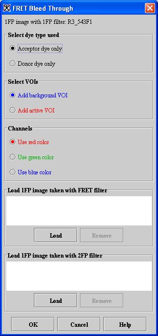
| 16:22, 31 July 2012 | DialogBoxFRETBleedThrough ColorImages.jpg (file) |  |
37 KB | Olga Vovk | FRET Bleed Through dialog box | 1 |
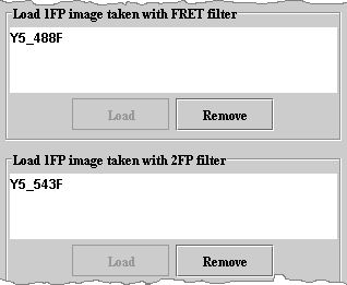
| 16:15, 31 July 2012 | LoadImageFRETBleedThrough.jpg (file) |  |
15 KB | Olga Vovk | The loaded images in the FRET Bleed Through dialog box | 1 |
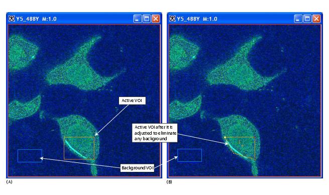
| 16:07, 31 July 2012 | FRET DonorRunVOIs7.jpg (file) |  |
48 KB | Olga Vovk | Donor only run: FP1 image with a background VOI in blue and an active VOI in orange (example image: Y5_488Y.tif) | 1 |
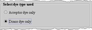
| 16:00, 31 July 2012 | DonorDyeOnly.jpg (file) |  |
7 KB | Olga Vovk | FRET Donor dye only selection | 1 |
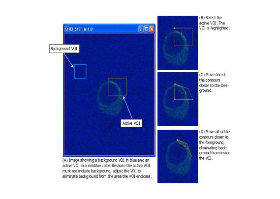
| 15:49, 31 July 2012 | ExampleFRET AcceptorRunVOIs11.jpg (file) |  |
24 KB | Olga Vovk | Acceptor only run: FP1 image with a background VOI in blue and an active VOI in orange (example image: R3_543F.tif) | 2 |
First page |
Previous page |
Next page |
Last page |