Interpolation methods used in MIPAV
Contents
Resampling
Resampling of an image is an important task in image analysis. The registration and transformation algorithms implemented in MIPAV resample images using an interpolation scheme, where anisotropic voxels (pixels for 2D images) are resampled into isotropic 1 mm cubic voxels. New voxel values are computed using a weighted combination of existing voxel values within a defined neighborhood of the new voxel location.
Because resampling is performed in space coordinates, it is important to preserve image spacing in the images involved. Interpolation is used because mapping from one image space to the other often requires evaluation of the intensity of the voxels at non-grid positions.
The following interpolation methods are available in MIPAV: Bilinear, Trilinear, B-spline 3-rd order, B-spline 4-th order, lagrange interpolations (including Cubic Lagrangian, Quintic Lagrangian, Heptic Lagrangian), Gaussian, and Windowed sinc.
Registration methods implemented in MIPAV
- B-Spline Automatic Registration
- Optimized automatic registration 3D
- Registration: Landmark-Least Squares
- Registration: Landmark-TPSpline
- Registration: Manual 2D Series
- Registration: Time Series Optimized Automatic Registration
Nearest-Neighbor
TBD.
Bilinear Interpolation
Bilinear interpolation considers the closest 2 x 2 neighborhood of known pixel values surrounding the unknown pixel. It then takes a weighted average of these 4 pixels to arrive at its final interpolated value. This results in smoother looking images. It performs linear interpolation in one direction, and then again in the other direction. Although each step is linear in terms of position and the sampled values the interpolation as a whole is not linear but rather quadratic in the sample location.
How to use
Bilinear interpolation can be used in transformations, where the perfect pixel matching is impossible, so one can calculate and assign appropriate intensity values to pixels. Unlike other interpolation techniques (e.g. nearest neighbor and bicubic interpolation), bilinear interpolation uses only the 4 nearest pixel values which are located in diagonal directions from a given pixel in order to find the appropriate color intensity values of that pixel.
Example
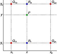
In the figure shown on your right, red dots Q12, Q22, Q11 and Q21 represent the known pixels and the green dot P is the pixel we wish to interpolate. Note that the known pixel distances are not equal.
To calculate the intensity for the green dot, we will first proceed with a linear interpolation in X direction and calculate intensity values for blue pixels R1 and R2, see Equation 1 and Equation 2.
<math> f(R_1) \sim \frac{x_2-x}{x_2 - x_1} f(Q_11) + \frac{x-x_1}{x_2 - x_1}f(Q_{21}), where R_1 = (x, y_1) </math>
<math> f(R_2) \sim \frac{x_2-x}{x_2 - x_1} f(Q_{12}) + \frac{x-x_1}{x_2 - x_1}f(Q_{22}), where R_2 = (x, y_2) </math>
Then, we will do interpolation in Y direction, see Equation 3.
<math> f(P) \sim \frac{y_2-y}{y_2 - y_1} f(R_1) + \frac{y-y_1}{y_2 - y_1}f(R_2) </math>
This gives us the desired interpolated value for the point <math>P=f(x,y)</math>, see Equation 4.
<math> f(x,y) \sim \frac{f(Q_{11})}{(x_2-x_1)(y_2 - y_1)}(x_2 - x)(y_2 - y) + \frac{f(Q_{21})}{(x_2-x_1)(y_2 - y_1)} (x - x_1) (y_2 - y) + \frac{f(Q_{12})}{(x_2-x_1)(y_2 - y_1)} (x_2 - x) (y - y_1) + \frac{f(Q_{22})}{(x_2-x_1)(y_2 - y_1)} (x - x_1)(y - y_1) </math>
Trilinear Interpolation
Trilinear interpolation computes intensity values for voxels with unknown intensity values, which are located between known voxel values. It does it by linearly weighting the eight closest neighboring values.
How to use
Trilinear interpolation is the default resampling interpolation method used in MIPAV registration techniques. In practice, a trilinear interpolation is identical to three successive linear interpolations, or two bilinear interpolations combined with a linear interpolation.
Example
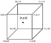
The figure on your right depicts the situation where it is desired to determine an intensity value at the point labeled (x, y, z), given the values at the corner of the cube. The unknown value is computed by combining the known corner values weight by their distance from the location of the point (x, y, z) according to the following formula:
<math>V_{xyz}</math> = <math>V_{000}</math> (1 - x) (1 - y) (1 - z) + <math>V_{100}</math> x (1 - y) (1 - z) + <math>V_{010}</math> (1 - x) y (1 - z) + <math>V_{001}</math> (1 - x) (1 - y) z + <math>V_{101}</math> x (1 - y) z + <math>V_{011}</math> (1 - x) y z + <math>V_{110}</math> x y (1 - z) + <math>V_{111}</math> x y z
B-spline basis interpolations
B-spline interpolation utilizes weighted voxel values in a larger neighborhood compared to trilinear interpolation. The larger number of values are weighted based on a 3-rd and 4-th order of polynomial, instead of a second order polynomial as in the case of trilinear interpolation. B-spline interpolation refers to the locations of the neighboring points as control points and combines the intensity values at these locations using a set of polynomial basis according to Equation 1.
The equation for k-order B-spline with n+1 control points (P0, P1, ... , Pn) is as follows:
<math> P(t) = \sum_{i=1}^{n+1} N_{i,k} (t) P_i, t_{min} \leq t < t_{max} </math>
In Equation 1, <math>N_{i,k}</math> are the polynomial functions of degree k-1, and n is the number of control points. Note, that the degree of the weighting polynomial is independent of the number of control points, n.
The weighting polynomial is recursively defined as
<math> N_{i,1} (t) = \left\{ \begin{array}{l l}
   1 & \quad  t_{i} \leq t < t_{i+1}\\
   0 & \quad otherwize\\
 \end{array} \right.
</math>
<math> N_{i,k} = \frac {t - t_{i}}{t_{i+k-1} - t_{i}} N_{i, k-1} (t) + \frac {t_{i+k} - t} {t_{i+k} - t_{i+1}} N_{i+1. k-1} (t) </math>
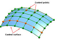
Here, t(i) represents an index that refer to the control points and t(i) are generally referred as knot points, see the figure on your right. The sequence of knot points is also called a knot vector. This indexing scheme allows one to weight different control points more than other control points by using it more than once during the computation. Typically, the first and last control points are weighed more heavily than the internal points to provide a smooth interpolating curve. The Optimized automatic registration 3D method uses the open uniform knot vectors for calculating B-splines. Open uniform knot vectors are vectors that have k equal knot values at each end, such as described in #EquationB3 Equation 3.
<math> \begin{array}{l l}
   t_i = t_1, i \leq k\\
   t_{i+1} - t _{i} = constant, k \leq i < n+2\\
   t_i = t _{k+(n+1)}, i \geq n+2\\
 \end{array}
</math>
How to use
B-splines are useful in those applications that consider image data as a continuum rather than a discrete array of pixels, for example when performing interpolations. Interpolation methods often perform various types of image registrations including intra-modal registration for rigid-body motion compensation, as well as inter-modal registration of CT, PET and MR data sets of a same subject. Another important area is visualization and operations like zooming, panning, rotation, reslicing and maximum intensity projection.
See also: Michael Unser, Splines: a perfect fit for medical imaging.
Example
For example: [0,0,0,0,1,2,3,4,4,4,4,] for k=4; [1, 1, 1, 2, 3, 4, 5, 6, 6, 6] for k=3; [0.1, 0.1, 0.1, 0.1, 0.1, 0.3, 0.5, 0.7, 0.7, 0.7, 0.7, 0.7] for k=5.
Gaussian
The Gaussian function is as follows:
<math> G(x) = \frac{1}{\sqrt{2\pi\sigma}}*exp -\frac {x^2}{2\sigma^2} </math>
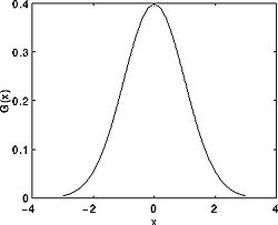
Where <math>\sigma</math> is the standard deviation of the distribution. We assume that the distribution has a mean of zero (i.e. it is centered on the line x=0). The distribution is illustrated in the Figure on your right.
In 2-D, an isotropic (i.e. circularly symmetric) Gaussian has the form:
<math> G(x) = \frac{1}{\sqrt{2\pi\sigma}}*exp -\frac {x^2 + y^2}{2\sigma^2} </math>
The idea of Gaussian interpolation is to use the 2-D distribution as a point-spread function, and this is achieved by convolution. Since the image is stored as a collection of discrete pixels the algorithm, first, produces a discrete approximation to the Gaussian function before it performs the convolution.
The Gaussian function is a recurrent with respect to operations such as derivation and Fourier transform.
Example
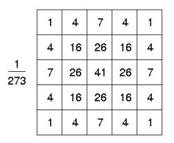
In theory, the Gaussian distribution is non-zero everywhere, which would require an infinitely large convolution kernel, but in practice it is effectively zero more than about three standard deviations from the mean, and so the algorithm truncates the kernel at this point. Figure on your right shows a suitable integer-valued convolution kernel that approximates a Gaussian with a sigma of 1.0.
Once a suitable kernel has been calculated, then the Gaussian interpolation can be performed using standard convolution methods. The convolution can be performed fairly quickly since equation 13 for the 2-D isotropic Gaussian shown above is separable into X and Y components. Therefore, the 2-D convolution can be performed by, first, convolving with a 1-D Gaussian in the Y direction, and then, convolving with another 1-D Gaussian in the Y direction. (The Gaussian is the only completely circularly symmetric operator which can be decomposed in such a way.) A further way to compute a Gaussian interpolation with a large standard deviation is to convolve an image several times with a smaller Gaussian.
Lagrange interpolations
To compute higher-order interpolations, the Optimized automatic registration 3D algorithm uses Lagrange interpolations. The Lagrange kernel of degree N-1 for an N x N region can be defined by Equation 1.
<math> Lagra_{h_{n}} (x) = \left\{ \begin{array}{l l}
\Pi_{j=0, j-N/2 +1 \neq n}^{N-1} \frac{n-i-x}{n-i}, n-1 \leq x < n \\
 0, elsewhare\\
\end{array} \right. </math>
Where i=j-N/2+1, and <math> n \in \{-N/2+1, -N/2+2, N/2\}</math>
Options provided by this method include the following Lagrange interpolations: Cubic (N = 3), quintic (N = 5), and heptic (N = 7).
The Lagrange kernel for N=1 is nearest neighbor interpolation. In the case N=2 it is linear interpolation. The Lagrange kernel for N=4 supporting points results in cubic polynomials, see Equation 2:
The Lagrange kernel for N=5 supporting points results in quadratic polynomials as shown in Equation 3:
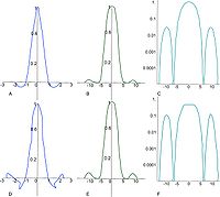
All Lagrange kernels are direct current (DC) constant. In other words, the mean brightness of the image is not affected if the image is interpolated or re-sampled. However, the even Lagrange interpolators do not fit C1-continuously at the connecting points causing significant sidelobes within their Fourier transforms. the Lagrange kernels for N=4 and N=5 are shown below.
- Lagra h4(x) shows a sharp edge at the center of the mask in the spatial domain. The amplitude of the sidelobe in the Fourier domain is about 4%.
- The odd Lagrange kernels, such as Lagra h5(x), is not C0-continuous.
Therefore, the amplitude of the sidelobe is raised up to 10% as shown in F (see figure (F)). However, the plateau in the passband is wider causing the major lobe to approximate more closely the ideal rectangular shape.
How to use
The passband characteristic is improved by raising the order of the Lagrange kernel (see figure). Therefore, odd Lagrange kernels, such as cubic (N = 3), quintic (N = 5), and heptic (N = 7), should be used for images with high contrasts.
Windowed sinc
The Windowed sinc function is a product of the sinc function with a window function of a limited spatial support. The sinc function can be defined as shown in Equation 1:
<math> sinc(x) = \left\{ \begin{array}{l l}
   \frac{sin(x)}{x} & \quad  \forall x \neq 0\\
   1 & \quad x=0 \\
 \end{array} \right.
</math>
Consider an image data set consisting of a 3D matrix of voxels with intensities I(X; Y; Z) identified by integer position coordinates (X; Y; Z). If one wants to calculate the intensity value at an interior point defined by non-integer coordinates (x; y; z), this can be achieved by forming the following triple sum, see Equation 2:
<math> I(x,y,z) = \sum_X \sum_Y \sum_Z i(X,Y,Z)sinc(\pi (x-X))sinc(\pi (y-Y))sinc(\pi (z-Z)) </math>
There are two limiting conditions that the function I(x, y, z) must satisfy:
- I(x, y, z) must be bandlimited. In other words, the function must have a Fourier transform F{I(x, y, z)}=I(f)=0 for |f|>B for some maximum frequency B>0.
- The sampling rate -fs, must exceed twice the bandwidth, e.g. fs >2B.
The interpolation formula reconstructs the original signal, I(interior), as long as these two conditions are met.
Equation 2 implies a sum over all voxels for each new intensity value calculated. Since this is computationally very demanding and since distant voxels (for which sinc weighting is small) make a little contribution, it is convenient in practical situations to truncate the interpolation series. This can be done by limiting the calculation to a cubic sub-volume containing (2R+2)3 voxels centered on the target point (x; y; z) for which an intensity is calculated. Here, R determines the size of the cubic box, and when R is zero only the eight nearest neighbors will be used in the calculation.
Because of the oscillating nature of the sinc function, some truncation errors and negative values may result from this procedure. To reduce the truncation error, each sinc function is multiplied by an apodizating the Hann window function, see Equation 3:
<math> H(\Delta; R)= \frac{1}{2}\Big[1+cos \big(\frac{\pi \Delta}{R+1}\big) \Big] </math>
The Windowed sinc interpolation, although very precise, are much slower than the linear and Gaussian interpolation.
References
- Thévenaz, Blu, and Unser, Interpolation Revisited, IEEE TRANSACTIONS ON MEDICAL IMAGING, VOL. 19, NO. 7, JULY 2000, Retrieved May 9, 2012
- Bourke Paul "Interpolation methods", ~pbourke/other/interpolation/index.html http://local.wasp.uwa.edu.au/ ~pbourke/other/interpolation/index.html, Retrieved May 9, 2012
- B-splines Web: http://www.cl.cam.ac.uk/teaching/1999/AGraphHCI/SMAG/node4.html, retrieved May 9, 2012
- Batchelor P. and Hill D. Chapter 3: "Registration Methodology: Concepts and Algorithms" in "Medical Image Registration", editors by Joseph V. Hajnal, Derek L.G.Hill, and David J. Hawkes, CRC Press, 2001, pp. 40-70.
- Woods R., Chapter 33 "Within-Modality Registration Using Intensity-Based Cost Functions" in "Handbook of Medical Image Processing and Analysis", Editor, Isaac N. Bankman, Academic Press, 2000, pp. 529-553.
- Lehmann Thomas M., Gonner C., and Spitzer K. Survey: Interpolation Methods in Medical Image Processing. IEEE TRANSACTIONS ON MEDICAL IMAGING, VOL. 18, NO. 11, NOVEMBER 1999 1049.
