Difference between revisions of "Interpolation methods used in MIPAV"
m (→Bilinear Interpolation) |
m (→Bilinear Interpolation) |
||
| Line 13: | Line 13: | ||
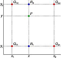
[[File:BilinearInterpolation.jpg|200px|thumb|right|Bilinear Interpolation - red dots show the known pixels and the green dot is the pixel we wish to interpolate]] | [[File:BilinearInterpolation.jpg|200px|thumb|right|Bilinear Interpolation - red dots show the known pixels and the green dot is the pixel we wish to interpolate]] | ||
| + | === Where to use === | ||
Bilinear interpolation can be used in transformations, where the perfect pixel matching is impossible, so one can calculate and assign appropriate intensity values to pixels. Unlike other interpolation techniques (e.g. nearest neighbor and bicubic interpolation), bilinear interpolation uses only the 4 nearest pixel values which are located in diagonal directions from a given pixel in order to find the appropriate color intensity values of that pixel. | Bilinear interpolation can be used in transformations, where the perfect pixel matching is impossible, so one can calculate and assign appropriate intensity values to pixels. Unlike other interpolation techniques (e.g. nearest neighbor and bicubic interpolation), bilinear interpolation uses only the 4 nearest pixel values which are located in diagonal directions from a given pixel in order to find the appropriate color intensity values of that pixel. | ||
| − | In the | + | === Example === |
| + | In the figure shown on your right, red dots Q12, Q22, Q11 and Q21 represent the known pixels and the green dot P is the pixel we wish to interpolate. Note that the known pixel distances are not equal. | ||
| − | To calculate the intensity for the green dot, we will first proceed with a linear interpolation in X direction and calculate intensity values for blue pixels R1 and R2 | + | To calculate the intensity for the green dot, we will first proceed with a linear interpolation in X direction and calculate intensity values for blue pixels R1 and R2, see [[#EquationOne | Equation 1]] and [[#EquationTwo | Equation 2]]. |
<div id="EquationOne">Equation 1</div> | <div id="EquationOne">Equation 1</div> | ||
| Line 31: | Line 33: | ||
</math> | </math> | ||
| − | Then, we will do interpolation in Y direction | + | Then, we will do interpolation in Y direction, see [[#EquationThree | Equation 3]]. |
<div id="EquationThree">Equation 3</div> | <div id="EquationThree">Equation 3</div> | ||
| Line 39: | Line 41: | ||
</math> | </math> | ||
| − | This gives us the desired interpolated value for <math>P=f(x,y)</math> | + | This gives us the desired interpolated value for the point <math>P=f(x,y)</math>, see [[#EquationFour | Equation 4]]. |
<div id="EquationFour">Equation 4</div> | <div id="EquationFour">Equation 4</div> | ||
Revision as of 18:35, 8 May 2012
This article is a stub. It needs improvement.
The registration and transformation algorithms implemented in MIPAV resampes images (if needed) using an interpolation scheme, where anisotropic voxels (or pixels for 2D images) are resampled into isotropic 1 mm cubic voxels. New voxel values are computed using a weighted combination of existing voxel values within a defined neighborhood of the new voxel location. The following interpolation methods are available in this implementation of the registration technique, including Bilinear, Trilinear, B-spline 3-rd order, B-spline 4-th order, Cubic Lagrangian, Quintic Lagrangian, Heptic Lagrangian, and Windowed sinc.
Bilinear Interpolation
Bilinear interpolation considers the closest 2 x 2 neighborhood of known pixel values surrounding the unknown pixel. It then takes a weighted average of these 4 pixels to arrive at its final interpolated value. This results in smoother looking images. It performs linear interpolation in one direction, and then again in the other direction. Although each step is linear in terms of position and the sampled values the interpolation as a whole is not linear but rather quadratic in the sample location.
Where to use
Bilinear interpolation can be used in transformations, where the perfect pixel matching is impossible, so one can calculate and assign appropriate intensity values to pixels. Unlike other interpolation techniques (e.g. nearest neighbor and bicubic interpolation), bilinear interpolation uses only the 4 nearest pixel values which are located in diagonal directions from a given pixel in order to find the appropriate color intensity values of that pixel.
Example
In the figure shown on your right, red dots Q12, Q22, Q11 and Q21 represent the known pixels and the green dot P is the pixel we wish to interpolate. Note that the known pixel distances are not equal.
To calculate the intensity for the green dot, we will first proceed with a linear interpolation in X direction and calculate intensity values for blue pixels R1 and R2, see Equation 1 and Equation 2.
<math> f(R_1) \sim \frac{x_2-x}{x_2 - x_1} f(Q_11) + \frac{x-x_1}{x_2 - x_1}f(Q_{21}), where R_1 = (x, y_1) </math>
<math> f(R_2) \sim \frac{x_2-x}{x_2 - x_1} f(Q_{12}) + \frac{x-x_1}{x_2 - x_1}f(Q_{22}), where R_2 = (x, y_2) </math>
Then, we will do interpolation in Y direction, see Equation 3.
<math> f(P) \sim \frac{y_2-y}{y_2 - y_1} f(R_1) + \frac{y-y_1}{y_2 - y_1}f(R_2) </math>
This gives us the desired interpolated value for the point <math>P=f(x,y)</math>, see Equation 4.
<math> f(x,y) \sim \frac{f(Q_{11})}{(x_2-x_1)(y_2 - y_1)}(x_2 - x)(y_2 - y) + \frac{f(Q_{21})}{(x_2-x_1)(y_2 - y_1)} (x - x_1) (y_2 - y) + \frac{f(Q_{12})}{(x_2-x_1)(y_2 - y_1)} (x_2 - x) (y - y_1) + \frac{f(Q_{22})}{(x_2-x_1)(y_2 - y_1)} (x - x_1)(y - y_1) </math>
See also: Optimized automatic registration 3D
