Filters (Spatial): Adaptive Path Smooth

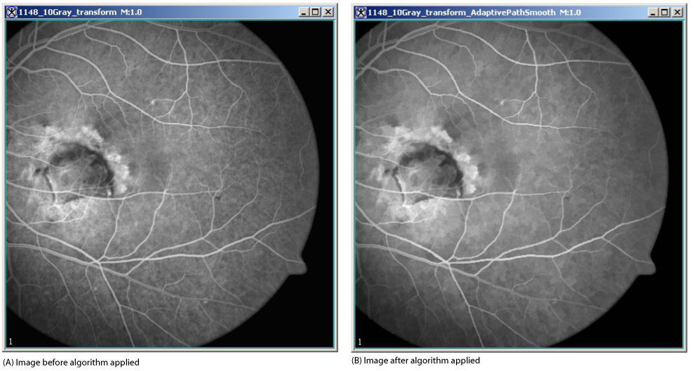
By replacing a pixel value with a weighted sum of the local pixels on the low-cost path, this algorithm reduces noise without blurring edges. It determines the weighted sum by following the path from the lowest-cost pixel at the edge of a local neighborhood back to the original pixel.

Background

MIPAV uses a modified port of image noise removal software by Karlis Freivalds for this algorithm. Freivalds' program starts by transforming RGB color space into YCrCb color space. After filtering is complete, the program then transforms the YCrCb color space back into RGB color space. Hence, all of the color operations occur in YCrCb space.

"Frequently Asked Questions about Color" by Charles Poynton reveals that the RGB-to-YCrCb and YCrCb-to-RGB conversion equations used in Freivalds' program differ significantly from the standard ones. Grayscale images are not transformed into another space.

In the original program as ported in the Adaptive Noise Reduction algorithm, the weighted sum was applied to all pixels in the () by () local square where range = (int)(radius 0.999). The program finds the lowest-cost pixel at the edge of the () by () local neighborhood. That pixel and the pixels along the low-cost path back to the original center pixel are the only pixels used in the weighted sum.

First, the program creates an edge graph or pixel neighbor graph. The 2D edge graph is an array of arrays with the first array having a length equal to the number of pixels in the image and the second array having eight edge weights. The eight edge weights are calculated from the intensity differences between the center pixel and one of the eight neighboring pixels.

In 2D and 2.5D images, the edge graph encompasses the entire image. In 3D with 26 nearest neighbors, an edge graph of size

<math> (2xrange+1)x(2xrange+1)x(2xrange+1)x26 </math>

is separately created for every voxel in the image to conserve memory.

For color images:

<math> E =\sqrt{((dYwY)^2 + (dRwR)^2 + (dBwB)^2)} </math>

where

EW = edge weight

dY, dR, and dB = Y, Cr, and Cb differences

wY, wR, and wB = Y, Cr, and Cb weights derived from the Y, Cr, and Cb radiuses

A bigger relative radius results in a smaller weight for radiuses >= 0.1, which should typically be the case. For grayscale images, edge weights are simply the absolute values of the differences between two pixels.

After the edge graph is created, the Y, Cr, and Cb spaces are separately filtered. The filter uses the selected pixel as the center of a square with sides of .

The function enhancePixel returns the filtered pixel value at every pixel in the image. If neighboring pixels are connected to the center pixel via a low-cost path, queue elements corresponding to these neighboring pixels are added to the priority queue. If no queue element is retrieved from the queue, then the original pixel value is passed unchanged. If elements are retrieved from the queue, then those Y, Cr, or Cb pixel values that retrieved queue elements in the path from the low-cost edge pixel to the center pixel are put into a weighted sum. The weight, derived from the distMap array, is simply the Gaussian function of the distance from the center pixel.

Each queue element has a value, a key, and an origin as indicated in the following:

• value = the location within the local ()*() local square
• key = sum of the edge graph values on the low-cost path from the center pixel to the selected pixel
• origin = the value of the queue element that provides the neighboring pixel on the low-cost path back to the center pixel with the center pixel origin = -1

A key is only added to the queue if an edge weight is less than threshold.

The priority queue is implemented as a binary heap and the binary heap is implemented as an array. A binary heap is a "nearly full" binary tree (only the bottom level may not be complete). This binary heap has the property that, for every node other than a leaf, its key value is less than or equal to that of its children. In a binary heap, the item of highest priority is always at the root of the tree or at node 0. When the highest priority item at the root is removed, the item of highest priority among the remainder moves into the root position. The children of node i are at and . The parent of node i is at <math> (int) \left ( \frac {i-1}{2} \right ) </math>.

Figure 1. Example of adaptive path smooth processing

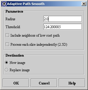
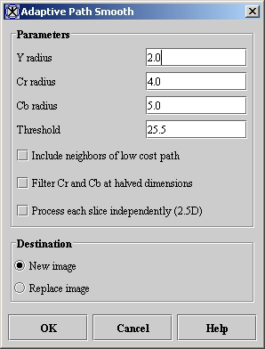
On the Adaptive Path Smooth dialog box for color images, you can separately adjust the filter radius for each Y, Cr, and Cb channel for color images. On the Adaptive Path Smooth dialog box for grayscale images, you can only adjust a single radius.

Tip: A larger radius removes more noise from the image but also loses more detail from the image.

You can also adjust the threshold for both color and grayscale images. Again, larger values preserve more edges but sacrifice smoothness in low-contrast areas. In addition, banding may appear for very large values.

For color images only, there is an option to filter Cr and Cb at halved dimensions. If this option is selected, the Cr and Cb spaces are shrunk by a factor of 2, an edge table is generated for the shrunken space, the filtering is performed, and the filtered Cr and Cb spaces are expanded back up to their original dimensions. The algorithm runs faster, but the image loses detail.

On both dialog boxes, if you choose New image, MIPAV then places the resulting image in a new image window. Selecting the Replace image option causes MIPAV to place the changed image in the same window.

Image types

You can apply this algorithm to both color and grayscale 2D and 3D images.

Special notes

None.

Reference

Refer to the following references for more information about this algorithm:

Image noise removal filter software by Karlis Freivalds at http://www.gradetools.com/karlisf

Frequently Asked Questions About Color by Charles Poynton at http://www.poynton.com/colorFAQ.html.

Applying the Adaptive Path Smooth algorithm

To run this algorithm, complete the following steps:

1. Open an image.
2. Select Algorithms > Filter(spatial) > Adaptive path smooth.

Depending on whether the image is grayscale or color, the Adaptive Path Smooth dialog box for grayscale images (Figure 2) or the Adaptive Path Smooth dialog box for color images opens. If the image is 3D, a check box to process each slice independently appears (Figure 3).

1. Complete the information in the dialog box.
2. Click OK.

The algorithm begins to run, and a progress bar appears with the status. When the algorithm finishes running, the progress bar disappears, and the results appear either in a new window or they replace the original source image.

Figure 2. Adaptive Path Smooth dialog box for grayscale images

Radius	The local square used is approximately (2 x Radius 1) times (2 x Radius 1) in size. As the radius increases the algorithm removes more noise but loses more details from the image. The default value is 2.0.
Threshold	Larger values preserve more edges but sacrifice smoothness in low-contrast areas. For very large values, banding may appear. The default value is 0.1 x (image maximum - image minimum).
Include neighbors of low cost path	Adds nearest neighbors of path pixels to the queue if they differ from the path pixels by less than threshold. However, the nearest neighbor weight is only half that of a path pixel. The default value is not selected.
Process each slice independently	Filters each slice of the dataset independently of adjacent slices. The default value is not selected. (This check box only appears for 3D images.)
New image	Shows the results of the algorithm in a new image window (default choice).
Replace image	Replaces the current active image with the new image produced by the algorithm.
OK	Applies the algorithm according to the specifications in this dialog box.
Cancel	Disregards any changes that you made in this dialog box and closes this dialog box.
Help	Displays online help for this dialog box.

Figure 3. Adaptive Path Smooth dialog box for 3D color images

Y radius	The local square used for Y space is approximately (2 x YRadius 1) times (2 x YRadius 1) in size. As the radius increases the algorithm removes more noise but loses more details from the image. The default value is 2.0.
Cr radius	The local square used for Cr space filtering is approximately (2 x CrR 1) x (2 x CrR 1) in size. As the radius increases, the algorithm removes more noise but loses more details from the image. The default value is 4.0.
Cb radius	The local square used for Cb space filtering is approximately (2 x CbR 1) x (2 x CbR 1) in size. As the radius increases, the algorithm removes more noise but loses more detail from the image. The default value is 5.0.
Threshold	Larger values preserve more edges but sacrifice smoothness in low-contrast areas. For very large values, banding may appear. The default value is 0.1 x (max (red max, green max, blue max) - min(red min, green min, blue min)).
Include neighbors of low cost path	Adds nearest neighbors of path pixels to the queue if they differ from the path pixels by less than threshold. However, the nearest neighbor weight is only half that of a path pixel. The default value is not selected.
Filter Cr and Cb at halved dimensions	When this option is selected, the algorithm runs faster but loses some detail. The default value is not selected.
Process each slide independently	Filters each slice of the dataset independently of adjacent slices. The default value is not selected. (This check box only appears for 3D images.)
New image	Shows the results of the algorithm in a new image window (default choice).
Replace image	Replaces the current active image with the new image produced by the algorithm.
OK	Applies the algorithm according to the specifications in this dialog box.
Cancel	Disregards any changes that you made in this dialog box and closes this dialog box.
Help	Displays online help for this dialog box.