Edge Detection: Zero X Non-Maximum Suppression

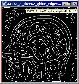
This method produces an edge map of the zero-crossings of the non-maximum suppression for 2D and 2.5D images. Edges are defined as the union of points for which the gradient magnitude assumes a maximum in the gradient direction.

Background

For a 2D image, let's introduce a local coordinate system (u, v) such that at any point in the image P0(x0,y0) v-axis is parallel to the gradient direction at (x0,y0) and the u-axis is perpendicular to it, i.e.,

Equation 1

<math> \binom {cos \alpha} {sin \alpha} = \frac {1} {\sqrt{L^2_x + L^2_y}} \binom {L_x} {L_y}_{(x_0;y_0)} </math>

Where L is a convolution of an image (represented as a function f(x,y) with the Gaussian kernel defined as:

Equation 2

<math> g(x,y) = \frac {1} {2\pi t}exp \left \{-\frac {x^2 +y^2} {2t} \right \} </math>

so that

Equation 3

<math> L{(x,y;t)} = g{(x,y;t)}of{(x,y)} </math>

where the circle represents convolution of g(x,y;t) and f(x,y) and semicolon in the argument of g implies that the convolution is performed only over the variables x and y, while the scale parameter t after the semicolon just indicates which scale-space level is being defined. Directional derivatives in this local (u,v) system are related to partial derivatives in the Cartesian coordinate system by the following system of equations,

Equation 4

<math> L_u = sin\alpha L_x - cos \alpha L_y </math> <math> L_v= cos\alpha L_x + sin\alpha L_y </math>

where, at a given point P0

Equation 5

<math> cos\alpha = \frac {L_x}{\sqrt{(L^2_x + L^2_y)}} </math>

<math> sin\alpha = \frac {L_y}{\sqrt{L^2_x + L^2_y}} </math>

And this (u,v) coordinate system is characterized by the fact that one of the two first-order derivatives -Lu, is zero, e.g.

Equation 6

<math> L_v = \frac {L^2_x + L^2_y}{\sqrt{L^2_x + L^2_y}} = {\sqrt{L^2_x + L^2_y}} </math>

Equation 7

<math> L_u= \frac {(L_xL_y - L_xL_y)}{\sqrt{(L^2_x + L^2_y)}} = 0 </math>

Equation 8

<math> L^2_v = L^2_x + L^2_y </math>

Below, are equations used in the method for calculating the second and third derivative - Lvv and Lvvv.

Equation 9

<math> L_{vv}=( cos\alpha L_x + sin\alpha L_y )^2 </math>

Equation 10

<math> L_{vv} = cos^2\alpha L_{xx} + 2cos\alpha sin\alpha L_{xy} + sin^2\alpha L_{yy} = \frac {L^2x L_{xx} + 2L_xL_yL_{xy} + L^2_yL_{yy}} {L^2_x + L^2_y} </math>

Equation 11

<math> L_{vvv} = \left ( cos^2 \alpha L_{xx} + \left ( 2 cos \alpha sin \alpha L_{xy} + sin \alpha^2 L_{yy} \right ) cos \alpha L_x + sin \alpha L_y \right ) = cos^3 \alpha L_{xxx} + 3cos^2 \alpha sin \alpha L_{xxy} +3cos \alpha sin^2 \alpha L_{xyy} + sin^3 \alpha L_{yyy} </math>

Equation 12

<math> L_{vvv} = \frac {L^3_x L_{xxx} + 3 L^2_x L_y L_{xxy} +3 L_x L^2_y L_{xyy} + L^3_y L_{yyy}} {(L^2_x +L^2_y)^{\frac {3} {2}}} </math>

Equation 13

<math> L^3_v L_{vvv} = L^3_x L_{xxx} + 3 L^2_x L_y L_{xxy} + 3 L_x L^2_y L_{xyy} +L^3 L_{yyy} </math>

According to the notion of non-maximum suppression, an edge point is defined as a point at which the gradient magnitude assumes a maximum in the gradient direction. In terms of directional derivatives, such definition can be also expressed as a combination of two conditions:

• • The second-order directional derivative in the v-direction Lvv being zero;
  • And the third-order directional derivative in the same direction Lvvv being negative, e.g.:

Equation 14

<math> \begin{cases} L_{vv} = 0,\\ L_{vvv} < 0 \end{cases} </math>

Since only the sign information is important, these conditions can be restated as:

Equation 15

<math> \begin{cases} L^2_v L_{vv} = 0\\ L^3 * L_{vvv} < 0 \end{cases} </math>

Here, L is the scale-space representation of an image f(x,y;t) at a certain scale t, and the last equation defines the edges of f at that scale.

This condition can also be formulated in terms of zero-crossings of the partial derivative of L with respect to the scale parameter (i.e., as a directional derivative in the vertical scale direction). For more information about the zero-crossings method for detecting edges used in MIPAV, refer to MIPAV User Manual, Volume 2, Algorithms, Edge Detection: Zero X Laplacian.

The method evaluates detected zero-crossings using the Marching Squares algorithm to determine only those zero-crossings that corresponds to edges. To learn more about the Marching Squares algorithm, refer to MIPAV User Manual, Volume 2, Algorithms, Extract Surface (Marching Cubes).

The resulting image is an unsigned byte image with values of 255 at the edges and 0 elsewhere.

Figure 1. The original image and its unsigned byte mask with detected edges.

Image types

You can apply this algorithm to 2D and 3D grayscale images.

References

Bart M. ter Haar Romeny(Ed.), "Geometry-Driven Diffusion in Computer Vision", Chapter2: Linear Scale'-'Space II: Early Visual Operations by Tony Lindeberg and Bart M. ter Haar Romeny, Kluwer Academic Publishers, 1994, pp. 39-46.

MIPAV User Manual, Volume 2, Algorithms, Edge Detection: Zero X Laplacian.

Tony Lindeberg [1996]. "Edge detection and ridge detection with automatic scale selection" Technical report ISRN KTH/NA/P-96/06-SE, May 1996, Revised August 1998. Int. J. of Computer Vision, vol 30, number 2, 1998. (In press). Shortened version in Proc. CVPR'96, San Francisco, June 1996. http://www.nada.kth.se/~tony

Applying the Zero X Non-Maximum Suppression algorithm

To run this algorithm, complete the following steps:

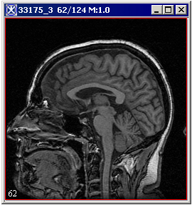
1. Open an image of interest;
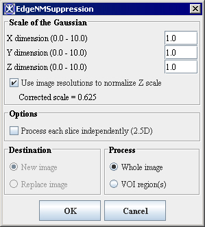
2. Select Algorithms > Edge detection > Zero x non-maximum suppression. The EdgeNMSuppression dialog box opens. For the dialog box options, refer to Figure 2.
3. Complete the fields in the dialog box. Click OK.

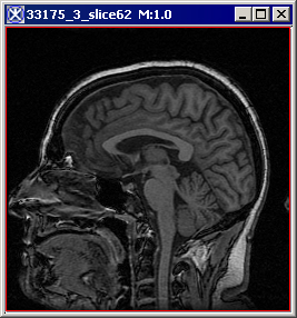
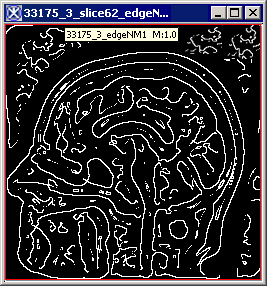
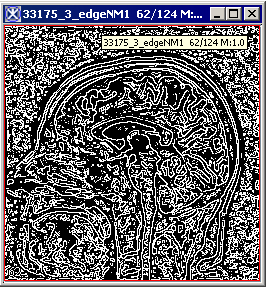
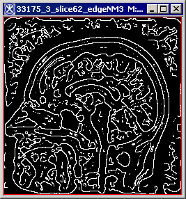
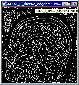
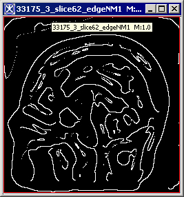
The algorithm begins to run, and a status window appears. When the algorithm finishes, the resulting image appears as an unsigned byte mask in a new image window as shown in Figure 3.

Figure 2. The EdgeNMSuppression dialog box options

Scale of the Gaussian	Specifies the standard deviation (from 1.0 to 10.0) of the Gaussian filter in X, Y, and Z directions which were used to determine edges in the image. Note that larger standard deviation produces an image with smaller number of edges. Smoothing the image before applying the algorithm also reduce the number of detected edges. Refer to Figure 3 for more information.
Use image resolutions to normalize Z scale	If checked, the following equation - Z scale*(X resolution/Z resolution) will be used to generate the edge map. If unchecked, only Z scale will be used in generation of the edge map.
Process each slice independently (2.5D)	Applies the algorithm to each image slice individually.
Destination	New image - this is the default option; Replace image - this option cannot be selected.
Process	Whole Image - if checked the edge detection will be calculated for the whole image; VOI region - if checked the edge detection will be calculated for the selected VOI.
OK	Applies the algorithm according to the specifications in this dialog box.
Cancel	Closes the dialog box.
Help	Displays online help for this dialog box.

Figure 3. The original image (a) and its unsigned byte mask with detected edges depending on the standard deviation: (b) - standard deviation is set to 1; (c) - standard deviation is set to 4; (d) - standard deviation is set to 6; (e) - standard deviation is set to 8; (f) - standard deviation is set to 6, but the original image has been smoothed before applying the algorithm.

a	b
c	d
e	f