B-Spline Automatic Registration

B-Spline Automatic Registration

This section describes the B-spline based registration of images in three dimensions (3D). The description specializes to two dimensions (2D) is in the obvious manner.

Background

Let the target image have dimensions with image indices satisfying , , and . Let the source image have dimensions with image indices satisfying , , and . The B-spline volume function maps indices via equation 1.

Equation 1

where the functions are the B-spline basis functions, and the B values are the control points. The numbers ,, and are user selectable, the degrees , , and for the basis functions are user selectable, and the B-spline basis functions are open and uniform.

The control points have the following characteristics:

• Each control point has coordinates from the unit cube. In two dimensions, each control point has coordinates from the unit square.
• The initial placement of the control points depends on the B-spline basis and must yield the identity function; that is, . The initial placement of the control points is described in Section [BSplineRegistrationOV_withMath.html#wp1000933 "Improving performance" ].
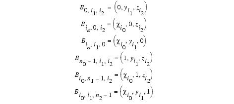
• A control point is said to be in the outer layer if one of its indexes is either the minimum index (zero) or the maximum index (one less than the number of control points in a given dimension). The position of the control points in the outer layer are fixed as follows:

Equation 2

This constraint implies that the ' 'for all .

• A control point not in the outer layer is said to be an interior control point. The position of the interior control points is constrained such that its movement must not cause any folding in the B-spline transformation. Folding is defined to occur when there is a negative value anywhere in the computed deformation for the current B-spline transformation. The computation of the deformation is described in Section [BSplineRegistrationOV_withMath.html#wp1001643 "Deformation" ]. The method by which folding is detected is described in Section [BSplineRegistrationOV_withMath.html#wp1001731 "Detect folding" ].

Each contains normalized 3D coordinates (i.e., in the unit cube) that identify a location in the source image corresponding to the sample at () in the target image. The coordinates are related to sample coordinates in the source image by where the output indices () are considered to be continuous values; that is, they are not necessarily integer valued. If the source image's samples are , where for all , we need to evaluate the image at the nonintegral values (). We can use trilinear interpolation to do this (use bilinear interpolation in the case of two-dimensional (2D) registration). Let , the largest integer smaller than . Define . The interpolated image value is:

Equation 3

If the target image samples are , where for all , then the source image is trilinearly interpolated at (), which are the coordinates of . This means that the currently registered source image, denoted , has the same dimensions as the target image and can be defined in terms of the target image samples as . A measure of error between the two images Sj0,j1,j2 and Tj0,j1 ,j2 can be computed. A number of possible error measure functions are defined in Section 1.2. The goal is to select the control point positions to make the error measure as small as possible. This is done by moving a single control point at a time using gradient descent.

The gradient of the error function is estimated for the control point Bi0,i1,i2 by means of finite differences, where changes in the error function are measured for small steps of the control point from its current position in each of the coordinate axis directions. Let , and be small step sizes equivalent to one sample increment in the target image,

Equation 4

The gradient of the error function is estimated at each control point Bi0,i1,i2. The gradient at each control point is denoted by

Equation 5

The gradient descent step is as follows. The current control point under consideration is Bi0,i1,i2. The ray originating at this point and having direction of greatest decrease in E is

Equation 6

where the direction is the unit length vector

and where is computed using equation 5. The idea is to choose t > 0 to minimize

A calculus approach which sets the first derivative to zero and solves for t yields an expression for e(t) that is really complicated. Instead, you should choose a set of t-values, t'1 through t'm, evaluate e(t'i') and find the minimum value. Suppose this occurs at t'k. Replace this in equation 6 to obtain the new location for the control point.

Only those t-values which do not result in the occurrence of folding in the B-spline transformation are considered. The method described in Section [BSplineRegistrationOV_withMath.html#wp1001731 "Detect folding" ] is used to determine if folding occurs for a given set of control point positions. Note that sample t0 (i.e., t=0) is equivalent to the location of the control point before any movement attempt, and by definition, sample t0 does not cause folding. A test is made to determine whether folding occurs for tm, the extreme sample in the set of chosen t-values. If folding does not occur at tm, then folding does not occur at any of the other t-values between t0 and tm. If folding does occur at tm, then a bisection method is employed to find the tf old value between t0 and tm where folding begins to occur. The search for a minimum value of e(t) by sampling must be limited to the t < t'f old.

Error measures

All of the error measures between two images defined in this section assume that the two images have the same dimensions. This is the case for the target image Tj'0 ',j'1',j'2' and registered source image S'`(j0,j1,j2) = S(k'`'0',k'`'1',k'`'2). The particular error measures defined here are only concerned with corresponding samples from the two images or histograms of the values of the samples from the two images, and are not concerned with whether the images have two or three dimensions. For simplicity, each image measure will be defined with a single index to access its samples.

Least squares measure

The least squares measure is defined by

Equation 7

where the summation is over all the indices for the target image voxels.

Here, S'`(j) is a registered source image and T(j) is a target image. The minimum value of this measure is zero; the maximum value depends on the range of values in the target and registered source images.

Correlation ratio measure

The correlation ratio measure is defined by

Equation 8

where

• Var(S) is the variance of the registered source image S.
• k is the number of intensity histogram bins equally distributed over the range of intensity values of the target image T.
• S'k'' is the k-th isoset defined as the set of intensities in registered source image S' at positions where the intensity in target image T is in the k-th intensity bin.
• nk is the number of elements in the set Sk, such that N =Sk ''n'k.
• N is the number of samples in the target image T which is the same number of samples in the registered source image S'.
• Var(Sk) is the variance of the values in the set Sk.

The range of values for this measure is [0,1].

Normalized mutual information measure

The normalized mutual information measure is defined by

Equation 9

where

is the standard entropy definition for probability pij estimated using the (i,j) joint histogram bins, and similarly for the marginals H(S') and H(T).

The standard entropy calculation

for an image X of N samples and user-selectable k histogram intensity bins equally distributed over the range of samples in image X can be rewritten as

where nk is the histogram value for the k-th intensity bin and N =S k nk. The computational effort can be reduced by factoring to get

where log n'k can be a precomputed lookup table of logarithms of integer values.

The range of values for this measure is [0,1].

Improving performance

The gradient descent applied to a control point at a time can be quite slow. Performance can be improved by taking advantage of the local control aspect of using B-splines. Since only one control point is being moved at a time, the local control aspect of using B-splines means that only some of the registered source image values will be different. Note that for an image of a given size, the number of image values, under local control, affected by moving a control point decreases as the number of control points increases.

One performance improvement can be achieved by precomputing the B-spline basis function values once for each possible sample for each dimension. Since the registration occurs by transforming the source image into the space of the target image, all samples for B-spline basis function evaluation always occur at the discrete sample coordinates for the target image. Since the number of target images samples for a dimension is xed, the B-spline basis function will be evaluated on the [0, 1] interval at equally spaced intervals (we are using open, uniform B-splines). For each dimension, a 2D array is created which stores B-splines basis function evaluations for each sample with the weight associated with each control point. Because of local control, many of these weights will be zero indicating that a sample is not affected by a particular control point. In the process of creating this 2D array of precomputed basis function evaluations, the index range of samples affected by each control point can be determined. The algorithm to determine this range does not examine the weights as they are computed; instead, the range of control points affecting a single sample are determined from the computed knot index and the known B-spline degree.

Another performance improvement involves maintaining intermediate error measure calculations. For example, in the case of the least squares error measure, an image is maintained of the current error calculations, that is, the target image subtracted from the current registered source image. A cumulative total error value is also maintained, which is the sum of the squared error values for all current values in the error image. When a control point is moved, the old values that are being replaced are first subtracted from the total error, and then the new values to be stored are added to the total error. Similar approaches are performed for the correlation ratio and normalized mutual information error measures such as storing cumulative histogram values and images which contain predetermined histogram bin indexes.

Initial placement of control points for identity map

Referring to equation 1 for the definition of the B-spline mapping function, the identity map is the one which yields

.

This section describes how to initially place the control points to yield this identity map. Since a separate set of B-spline basis functions is defined for each dimension, it happens that the placement of the control points to provide this identity map is computed independently for each dimension. This means that the x-coordinate for each control point initially is determined by the B-spline basis defined for the X-axis, and similarly for other dimensions.

Let k be the coordinate for which the control point identity map is being computed for the associated B-spline basis. Let nk be the number of control points defined for that B-spline basis. Let ik be the index of the control point coordinate such that 0<= ik <= nk. The goal is to compute the coordinate values Bik for all ik where each coordinate value is in the [0,1] range.

For a B-spline basis of degree 1, the initial placement of the control points for the identity map is such that the control point coordinates are uniformly spaced as follows:

Equation 10

for coordinate k. If the problem is to register images of three dimensions, and the B-spline bases for all three dimensions are selected to have degree 1, then

Equation 11

For a B-spline basis of degree 2 or larger, the initial placement of the control point coordinates is computed by the method of least squares. Again referring to [BSplineRegistrationOV_withMath.html#wp1012563 equation 2] for the definition of the B-spline mapping function, the identity map for coordinate k is

for any target image coordinate jk satisfying 0<= jk <pk.

A system of pk equations above for nk 1 unknowns (i.e., the Bik coordinate values) is set up in a matrix form AX = C, where

The solution is computed as

The repositioning of the control points to yield this identity map is guaranteed not have create folding in the resulting transformation.

Composition for two-pass registration

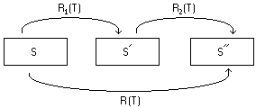
Let S be a source image and T be the target image. If the image S is registered to image T, then image S becomes the registered source image where R(T) is the registration mapping. This is graphically shown as:

For B-spline registration, the R(T) mapping is based on the selected B-spline basis and control points for each axis.

In the case of two-pass registration, the registered source image S' is then registered to the same target image T, but this time using different mapping parameters, i.e., a different set of B-spline basis and control points for the axes. The output of this second registration is a new registered source image S". Let R'1'(T) be the mapping for the first pass registration and R'2'(T) be the mapping for the second pass registration. This is graphically shown as:

The usefulness of a two-pass registration is that the first pass would apply a coarse-level computation to quickly arrive at an approximate registration, and then the second pass would apply a finer-level computation to continue from the point where the first pass registration finished. The first pass registration may use B-spline bases with fewer control points and a smaller degree.

Although the two-pass registration can be performed in the manner just described, it is desirable to have a final registration between the original source image S and the target image T.

This means defining a mapping R(T) having the same B-spline bases as the second pass registration mapping R'2'(T), but which maps the original source image S into the final registered source image S. This is graphically shown as:

The R(T) mapping for the second pass in a two-pass registration is different in that the initial placement of the control points does not yield the identity map to the original source image S.

Instead, the initial placement of the control points for R(T) yields the output of the R'1'(T) mapping. This is achieved by initializing the R'2'(T) registration mapping in the normal manner which provides an initial placement of its control points to yield the identity map from the registered source image S. The initial placement of the control points for the R(T) mapping then are the initial placement of the control points for R'2'(T) mapped through R'1'(T).

Deformation

The deformation from the nonlinearly registered source image S to the target image T can be measured at each sample in the target image by computing the determinant of the Jacobian matrix for the nonlinear transformation. For three dimensions, the nonlinear registration transformation is defined by equation 1. Since each Mj0j1j2 contains normalized 3D coordinates of the position in the source image mapped for each (j0, j1, j2) in the target image, a map image of 3D coordinates can be created that contains these Mj0j1j2 source images coordinates (this map image has the same dimensions as the target image). An estimate of the gradient at each sample in this map image is computed using central finite differences at interior samples and forward/backward finite differences at "outer layer" samples. Since each sample in the map image contains 3D coordinates, the estimated gradient at each sample then is a 3x3 matrix of values representing the Jacobian matrix. A single-valued deformation image with the same dimensions as the target image is created which contains the computed determinants of the Jacobian matrices for each sample.

If no deformation has occurred at a sample, the Jacobian matrix is the identity and its determinant is 1. If the source image is compressed near a sample, the determinant will be less than one. If the source image is expanded near a sample, the determinant will be greater than one. The computation of deformation is unaffected by differences in the dimensions for the source and target images. Because of the constraints on the placement of the control points, a negative determinant should not be possible, which would indicate some type of folding in the mapping.

Detect folding

The situation of folding in a 2D or 3D B-spline transformation occurs when there is a negative value in the computed deformation. The computation of the deformation is described in Section [BSplineRegistrationOV_withMath.html#wp1001643 "Deformation" ]. This section describes a method for detecting if such folding occurs given the current positions for the lattice of the B-spline control points. Given the lattice structure of the B-spline control points, folding can be detected by geometric means. In two dimensions, consider any interior control point and its 8 neighboring control points forming a polygon. Construct 8 triangles involving the chosen interior control point each time with the 8 pairings of adjacent control points on the polygon perimeter. The intersection of any one triangle with the other 7 triangles should each be empty in order for there to be no folding. Alternatively, the area of the polygon should be identical to the union of the areas of the 8 triangles.

The issues are similar in three dimensions by considering the 26 neighboring control points forming a polyhedron. In this case, 48 tetrahedrons are constructed involving the chosen interior control point each time along with the triples of control points from the 48 triangles forming the polyhedron mesh. The intersection of any one tetrahedron with the other 47 tetrahedrons should each be empty in order for there to be no folding. Alternatively, the volume of the polyhedron should be identical to the union of the volumes of the 48 tetrahedrons.

A sufficient but not necessary condition to conclude that folding occurs in the case of two dimensions is the premise that any interior control point is outside the polygon formed by its 8 neighboring control points. In the case of three dimensions, the premise is that any interior control point is outside the polyhedron formed by its 26 neighboring control points.

A condition that is both necessary and sufficient to conclude that folding occurs does exist for both 2D and 3D. In the case of two dimensions, again consider the 8 triangles formed by the chosen interior control point each time with the 8 pairings of adjacent control points on the polygon perimeter. It is important that these triangles formed by control points from the lattice be consistently counterclockwise ordered. For each triangle, let A =(a0,a1) be the 2D coordinates of the chosen interior control point, and let B =(b0,b1) and C =(c0,c1) be the 2D coordinates of the other two triangle control points taken in counterclockwise order. The normal to the plane which contains this triangle can be computed from the (right handed) cross product of the two vectors AB and AC. One way to express the calculation of the cross product involves the construction of the following matrix which contains the three triangle point coordinates:

Equation 12

The determinant of this matrix is twice the signed area of the triangle. Starting with consistently counter clockwise ordered triangles from the initially placed lattice of control points, the determinant of this matrix should remain positive as control point positions are moved. The determinant will become negative when the triangle folds.

The premise for the necessary and sufficient condition to detect when folding occurs extends to three dimensions. Consider the 48 tetrahedrons formed by the chosen interior control point each time with the triples of adjacent control points from the 48 triangles forming the polyhedron mesh. It is important that the tetrahedrons formed by the control points from the lattice be consistently counterclockwise ordered, in the 3D sense. For each tetrahedron, let A = (a0,a1,a2) be the 3D coordinates of the chosen interior control point, and let B = (b0,b1,b2), C = (c0,c1,c2), and D = (d0,d1,d2) be the 3D coordinates of the other three tetrahedron control points taken in counterclockwise order. Extending the matrix determinant formulation used for two dimensions to three dimensions, the following matrix is constructed which contains the four tetrahedron point coordinates:

The determinant of this matrix is 6 times the signed volume of the tetrahedron. Starting with consistently counterclockwise ordered tetrahedrons from the initially placed lattice of control points, the determinant of this matrix should remain positive as control point positions are moved. The determinant will become negative when the tetrahedron folds.

Support for color images

The registration of 2D and 3D color images involves first converting the three color channels of values at each sample in the source and target color images to create single channel source and target intensity images. Once the conversion has been done, the single channel intensity source and target images are registered as described in Background. The resulting transformation map is extracted from the registration which is then used to interpolate the original source color image in order to generate the output registered source color image.

Normally, the three color channels represent red, green, and blue intensities, and so the conversion to a single channel value usually represents overall intensity. In this manner, the conversion is simply a weighted average of the three color channels where separate weights can be provided for each channel. The current implementation uses equal weights for each channel.

Support for 2.5D images

A 2.5D image is actually a 3D image containing a series 2D slice images. The registration of a 2.5D intensity or color image involves a 2D registration of each slice in the 2.5D image to a reference slice also in the same 2.5D image. The reference slice can either be a xed slice or the previous slice. The resulting output registered 2.5D image contains the same number of slices as the original 2.5D image where the sample values in a slice of the registered output are from the same slice of the original only "warped" by the B-spline registration transformation.

If the reference slice is fixed, then the reference slice will appear in the registered output as being unchanged. If the reference slice is the previous slice, then the first slice will be registered to the last slice.

Examples of B-spline registration

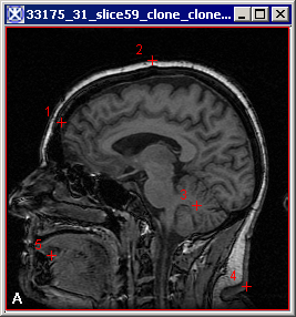
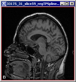
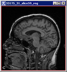
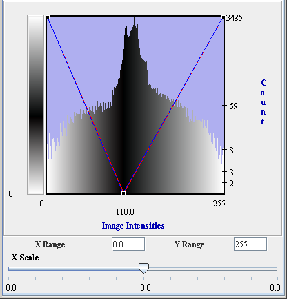
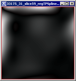
Figure 1 below shows an example of B-spline 3D image registration. [[BSplineRegistrationOV_withMath.html#wp1018286 |Figure 2] shows the registration deformation image and its lookup table. The registration was done using the default parameter values, which are explained in Section Image types.

Note: that the input and the target image are both images of the same brain, that's why the registration demonstrates a very good overall fitting.

Figure 1. The input source image (A), the input target image (B) and the output registered image (C). Note that images (A) and (B) are both the images of the same brain. That's why it shows a very good overall fitting. Results may vary, if you take different brain images.

Figure 2. The deformation image and its lookup table. The dark areas on the deformation image are related to the areas on images (A) and (B) which did not perform a deformation during the registration or the deformation was relatively small. The light areas are related to the areas on images (A) and (B) which perform a bigger deformation.

Image types

The algorithm can be applied to 2D and 3D color (RGB) and grayscale images.

User Dialogs in MIPAV

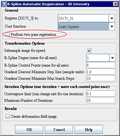
Whenever B-spline registration is selected by the user, a dialog is displayed for the user to select the registration reference and the options related to how the registration is to be performed. A different dialog is displayed depending on whether the user selects 2D/3D registration between two images, or 2.5D registration of slices within a single image. The displayed dialogs differ only in how the registration reference is specified which depends on whether 2D/3D registration or 2.5D registration was selected; otherwise, options related to how the registration is to be performed are the same.

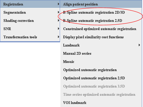
The choice of 2D/3D or 2.5D B-spline registration is made by selecting the appropriate menu item from the Algorithms: Registration submenu of MIPAV. Refer to Figure 3 for details.

Figure 3. The choice of 2D/3D or 2.5D B-spline registration is made by selecting the appropriate menu item from the Algorithms: Registration submenu

The 2D/3D B-spline registration is available through the B-spline automatic registration 2D/3D menu item. This menu item is enabled when a 2D or 3D image (intensity or color) is the currently active image. The dialog is displayed only if there is at least one other loaded image in MIPAV which is compatible for registering to the currently active image. A compatible image is one that has the same number of channels of data and the same number of dimensions, but not necessarily the same sizes for each dimension. Refer to Figures 4 and 5. The 2.5D B-spline registration is available through the B-spline automatic registration 2.5D menu item. This menu item is enabled only when a 3D image (intensity or color) is the currently active image. Refer to Figure 6. Since the options related to how the registration is to be performed are identical for 2D/2.5D/3D and intensity/color images, and the only difference is how the registration reference is selected for 2D/3D vs. 2.5D, the dialog for presenting these options to the user is implemented in the same class. This class is JDialogRegistrationBSpline and is in the mipav/model/view/dialogs package. The class dynamically creates a dialog to present to the user with options that are appropriate for the type of registration.

B-Spline Single - Pass Automatic Registration 2D/3D dialog box

Figure 4. B-Spline Single - Pass Automatic Registration 2D/3D dialog box

General
Register	Displays a list of currently active 2D/3D images to registration. The drop down list of options show the names of available images currently loaded to which this image can be registered. This list will only contain the names of images currently loaded in MIPAV which are compatible.	<
Cost function	This drop down list contains the following choices for cost measure to use during registration: Least Squares, Correlation Ratio, and Normalized Mutual Information.
Perform two-pass registra-tion	This dialog is shown with the default options for single-pass registration. If the Perform two-pass registration option is enabled, then the dialog will change to make options for two-pass registration available.
Transformation Options The following is a discussion of the dialog options which control each registration pass, one set of options per pass. For more information refer to Transformation options
Sub-sample image for speed	If this option is enabled, the image will be subsample in power of 2 for each dimension. Subsampling increases performance of the algorithm, but it exhibits lower accuracy of registration.
B-Spline Degree (same for all axes)	This is the degree of the B-Spline to use for all axes of the image. The drop list of options show the values of 1 (linear), 2 (quadratic), 3 (cubic), and 4 which are available. Although, the underlying BSpineBasisf class supports any degree, this dialog restricts the degrees to these values. Choosing a smaller degree executes faster than a larger degree, but a higher degree offers a higher order of continuity.
B-Spline Control Points(same for all axes)	This is the number of B-spline control points to use for all axes of the image.The minimum number of control points is the larger of the number 2 and the degree of the B-Spline. This dialog limits the maximum number of control points to one-half of the number of samples in the smallest dimension.
Gradient Descent Minimize Step Size (sample units)<a name="wp1022724"></a>	This is the size of steps each control point is moved along the gradient-based direction when searching for a minimum of the error. The registration does not take into account the size of an image sample in each dimension, so this step size is specified in units of a sample. E.g., a value of 0.5 will move the control point in increments of half of a sample while searching for the minimum error. The minimum step size is 0.1 sample and the maximum is 5 samples.
Gradient Descent Minimize Max Search Steps	This is the maximum number of steps the control point is moved along the gradient-based direction when searching for a minimum of the error. If the distance from the control point current position to the bounding polygon/polyhedron of its neighboring control points along the gradient-based direction is less than this specified value, then the computed distance value will be used for this control point instead. The minimum number of steps is 1 and the maximum is 100.<
Iteration options (one iteration=move each control point once)
Convergence limit (min change rate for one iteration)		This is a rate of change threshold such that if the rate the error changes between starting and ending of each iteration is smaller than this value, then the registration terminates.
Maximum Number of Iterations		If the convergence limit is not satisfied after this many iterations have been executed, then the registration terminates. The range of possible values is 1 to 100.
Results
Create deforma-tion field image	If this checkbox is enabled, then the deformation image is computed after the last pass of registration is performed. The image that is created has the same dimensions as the target and the registered source images, and has the name of the source image appended with deformation suffix. The deformation image will be automatically displayed along with the registered source image upon completion of registration. Refer to Figure5 for details.
<b>OK</b>	Applies the algorithm to the input image that you chose in this dialog box.
<b>Cancel</b>	Disregards any changes that you made in this dialog box and closes the dialog box.
<b>Help</b><	Displays online help for this dialog box.</a>

Figure 5. B-Spline Two - Pass Automatic Registration 2D/3D dialog box

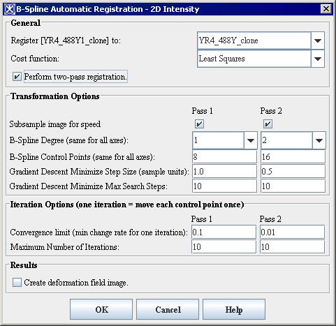
If the Perform two-pass registration check box is selected, then the dialog will change to the following:

General
Register	Displays a list of currently active 2D/3D images to registration. The drop down list of options show the names of available images currently loaded to which this image can be registered. This list will only contain the names of images currently loaded in MIPAV which are compatible.
Cost function	This drop down list contains the following choices for cost measure to use during registration: Least Squares, Correlation Ratio, and Normalized Mutual Information.
Perform two-pass registra-tion	This dialog is shown with the default options for two-pass registration. If the Perform two-pass registration option is disabled, then the dialog will change to make options for single-pass registration available as shown in Figure 4
Transformation Options The following is a discussion of the dialog options which control each registration pass, one set of options per pass. For more information refer to <a Transformation options
Sub-sample image for speed	If this option is enabled, the image will be subsample in power of 2 for each dimension. Subsampling increases performance of the algorithm, but it results lower accuracy of registration.
B-Spline Degree (same for all axes)	This is the degree of the B-Spline to use for all axes of the image. The drop list of options show the values of 1 (linear), 2 (quadratic), 3 (cubic), and 4 which are available. Although, the underlying BSpineBasisf class supports any degree, this dialog restricts the degrees to these values. Choosing a smaller degree executes faster than a larger degree, but a higher degree offers a higher order of continuity.
B-Spline Control Points(same for all axes)	This is the number of B-spline control points to use for all axes of the image.The minimum number of control points is the larger of the number 2 and the degree of the B-Spline. This dialog limits the maximum number of control points to one-half of the number of samples in the smallest dimension.
Gradient Descent Minimize Step Size (sample units)	This is the size of steps each control point is moved along the gradient-based direction when searching for a minimum of the error. The registration does not take into account the size of an image sample in each dimension, so this step size is specified in units of a sample. E.g., a value of 0.5 will move the control point in increments of half of a sample while searching for the minimum error. The minimum step size is 0.1 sample and the maximum is 5 samples.
Gradient Descent Minimize Max Search Steps	This is the maximum number of steps the control point is moved along the gradient-based direction when searching for a minimum of the error. If the distance from the control point current position to the bounding polygon/polyhedron of its neighboring control points along the gradient-based direction is less than this specified value, then the computed distance value will be used for this control point instead. The minimum number of steps is 1 and the maximum is 100.
Iteration options (one iteration=move each control point once)
Convergence limit (min change rate for one iteration)		This is a rate of change threshold such that if the rate the error changes between starting and ending of each iteration is smaller than this value, then the registration terminates.
Maximum Number of Iterations		If the convergence limit is not satisfied after this many iterations have been executed, then the registration terminates. The range of possible values is 1 to 100.
Results
Create deforma-tion field image	If this checkbox is enabled, then the deformation image is computed after the last pass of registration is performed. The image that is created has the same dimensions as the target and the registered source images, and has the name of the source image appended with deformation suffix. The deformation image will be automatically displayed along with the registered source image upon completion of registration. Refer to Figure 5for details.
OK	Applies the algorithm to the input image that you chose in this dialog box.
Cancel	Disregards any changes that you made in this dialog box and closes the dialog box.
Help	Displays online help for this dialog box.

This dialog is shown with the default options for a two-pass registration. As previously mentioned and as indicated in the dialog, a single iteration involves the movement of each interior control point in a gradient descent minimization manner.

<a name="wp1003337"></a></p>

B-Spline Single - Pass Automatic Registration 2.5D dialog box

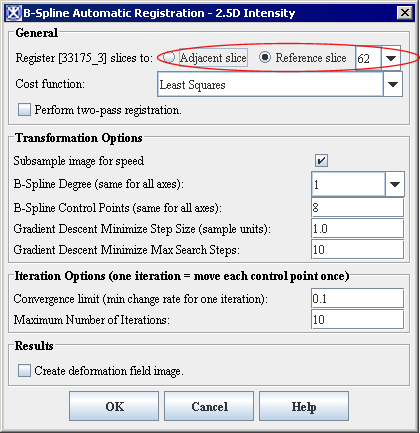
The following is an example of the dialog which is displayed for 2.5D intensity/color image registration: This dialog is show with the default options for a single-pass registration. If the Perform two-pass registration check box is selected, then the dialog will change in a manner similar to that for the 2D/3D image registration shown in Figure 5.

Figure 6. B-Spline Single - Pass Automatic Registration 2.5D dialog box

General
Register	The Register source field is already filled with the name of the currently selected 2.5D image. The reference slice is selected from among the slices in the selected image. Radio buttons are used to select whether the reference slice is the the adjacent (previous) slice or a particular slice number in the image. If the Reference Slice radio button is selected, then a drop down list of slices numbers is enabled where the middle slice is selected by default.
Cost function	This drop down list contains the following choices for cost measure to use during registration: Least Squares, Correlation Ratio, and Normalized Mutual Information.
Perform two-pass registration	This dialog is shown with the default options for single-pass registration. If the Perform two-pass registration option is enabled, then the dialog will change to make options for two-pass registration</em> available. Refer to Figure 7
Transformation Options The following is a discussion of the dialog options which control each registration pass, one set of options per pass. For more information refer to Transformation options.
Sub-sample image for speed	If this option is enabled, the image will be subsample in power of 2 for each dimension. Subsampling increases performance of the algorithm, but it results lower accuracy of registration.
B-Spline Degree (same for all axes)	This is the degree of the B-Spline to use for all axes of the image. The drop list of options show the values of 1 (linear), 2 (quadratic), 3 (cubic), and 4 which are available. Although, the underlying BSpineBasisf class supports any degree, this dialog restricts the degrees to these values. Choosing a smaller degree executes faster than a larger degree, but a higher degree offers a higher order of continuity.
B-Spline Control Points(same for all axes)	This is the number of B-spline control points to use for all axes of the image.The minimum number of control points is the larger of the number 2 and the degree of the B-Spline. This dialog limits the maximum number of control points to one-half of the number of samples in the smallest dimension.
Gradient Descent Minimize Step Size (sample units)	This is the size of steps each control point is moved along the gradient-based direction when searching for a minimum of the error. The registration does not take into account the size of an image sample in each dimension, so this step size is specified in units of a sample. E.g., a value of 0.5 will move the control point in increments of half of a sample while searching for the minimum error. The minimum step size is 0.1 sample and the maximum is 5 samples.
Gradient Descent Minimize Max Search Steps	This is the maximum number of steps the control point is moved along the gradient-based direction when searching for a minimum of the error. If the distance from the control point current position to the bounding polygon/polyhedron of its neighboring control points along the gradient-based direction is less than this specified value, then the computed distance value will be used for this control point instead. The minimum number of steps is 1 and the maximum is 100.
Iteration options (one iteration=move each control point once)
Convergence limit (min change rate for one iteration)		This is a rate of change threshold such that if the rate the error changes between starting and ending of each iteration is smaller than this value, then the registration terminates.
Maximum Number of Iterations		If the convergence limit is not satisfied after this many iterations have been executed, then the registration terminates. The range of possible values is 1 to 100.
Results
Create deformation field image	If this checkbox is enabled, then the deformation image is computed after the last pass of registration is performed. The image that is created has the same dimensions as the target and the registered source images, and has the name of the source image appended with deformation suffix. The deformation image will be automatically displayed along with the registered source image upon completion of registration. Refer to Figure 2 for details.
OK	Applies the algorithm to the input image that you chose in this dialog box.
Cancel	Disregards any changes that you made in this dialog box and closes the dialog box.
Help	Displays online help for this dialog box.

B-Spline Two - Pass Automatic Registration 2.5D dialog box

Figure 7. B-Spline Two - Pass Automatic Registration 2.5D dialog box

General
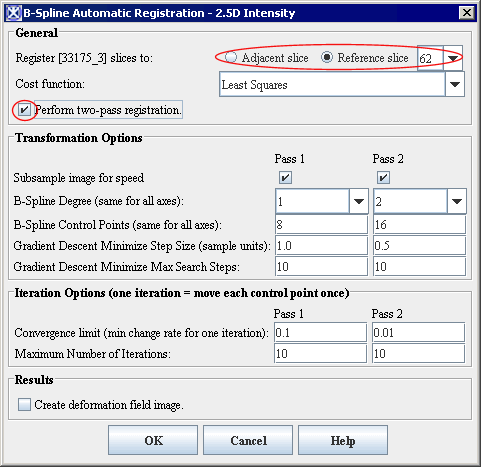
Register	The Register source field is already filled with the name of the currently selected 2.5D image. The reference slice is selected from among the slices in the selected image. Radio buttons are used to select whether the reference slice is the the adjacent (previous) slice or a particular slice number in the image. If the Reference Slice radio button is selected, then a drop down list of slices numbers is enabled where the middle slice is selected by default.
Cost function	This drop down list contains the following choices for cost measure to use during registration: Least Squares, Correlation Ratio, and Normalized Mutual Information.
Perform two-pass registration<		This dialog is shown with the default options for two-pass registration.
Transformation Options The following is a discussion of the dialog options which control each registration pass, one set of options per pass. For more information refer to Transformation options.
Sub-sample image for speed	If this option is enabled, the image will be subsample in power of 2 for each dimension. Subsampling increases performance of the algorithm, but it results lower accuracy of registration.
B-Spline Degree (same for all axes)	This is the degree of the B-Spline to use for all axes of the image. The drop list of options show the values of 1 (linear), 2 (quadratic), 3 (cubic), and 4 which are available. Although, the underlying BSpineBasisf class supports any degree, this dialog restricts the degrees to these values. Choosing a smaller degree executes faster than a larger degree, but a higher degree offers a higher order of continuity.
B-Spline Control Points(same for all axes)	This is the number of B-spline control points to use for all axes of the image.The minimum number of control points is the larger of the number 2 and the degree of the B-Spline. This dialog limits the maximum number of control points to one-half of the number of samples in the smallest dimension.
Gradient Descent Minimize Step Size (sample units)	This is the size of steps each control point is moved along the gradient-based direction when searching for a minimum of the error. The registration does not take into account the size of an image sample in each dimension, so this step size is specified in units of a sample. E.g., a value of 0.5 will move the control point in increments of half of a sample while searching for the minimum error. The minimum step size is 0.1 sample and the maximum is 5 samples.
Gradient Descent Minimize Max Search Steps	This is the maximum number of steps the control point is moved along the gradient-based direction when searching for a minimum of the error. If the distance from the control point current position to the bounding polygon/polyhedron of its neighboring control points along the gradient-based direction is less than this specified value, then the computed distance value will be used for this control point instead. The minimum number of steps is 1 and the maximum is 100.
Iteration options (one iteration=move each control point once)
Convergence limit (min change rate for one iteration)		This is a rate of change threshold such that if the rate the error changes between starting and ending of each iteration is smaller than this value, then the registration terminates.
Maximum Number of Iterations		If the convergence limit is not satisfied after this many iterations have been executed, then the registration terminates. The range of possible values is 1 to 100.
Results
Create deformation field image	If this checkbox is enabled, then the deformation image is computed after the last pass of registration is performed. The image that is created has the same dimensions as the target and the registered source images, and has the name of the source image appended with deformation suffix. The deformation image will be automatically displayed along with the registered source image upon completion of registration. Refer to Figure 2 for details.
OK	Applies the algorithm to the input image that you chose in this dialog box.
Cancel	Disregards any changes that you made in this dialog box and closes the dialog box.
Help	Displays online help for this dialog box.

Transformation options

The following is a discussion of the dialog options which control each registration pass, one set of options per pass:

B-spline Degree (same for all axes): This is the degree of the B-spline to use for all axes of the image. Even though the BSplineRegistration2Df and BSplineRegistration3Df classes allow for specification of separate degrees for each axis, this dialog restricts the degrees to be the same. The drop list of options show the values of 1 (linear), 2 (quadratic), 3 (cubic), and 4 which are available. Although, the underlying BSpineBasisf class supports any degree, this dialog restricts the degrees to these values.Choosing a smaller degree executes faster than a larger degree, but a higher degree offers a higher order of continuity.

B-spline Control Points (same for all axes): This is the number of B-spline control points to use for all axes of the image. Even though the BSplineRegistration2Df and BSplineRegistration3Df classes allow for specification of separate number of control points for each axis, this dialog restricts the numbers of control points to be the same. Initially, the control points are evenly spaced in each dimension, and the registration algorithm moves the interior control points to minimize the error difference between the target image and the registered source image. The minimum number of control points is the larger of the number 2 and the degree of the B-spline. This dialog option limits the maximum number of control points to one-half of the number of samples in the smallest dimension. Choosing more control points generally results in better overall fitting, but a limitation may be that the control points will be closer to each other and that will limit how much a control point can move to minimize the error (in order to satisfy the constraint that an interior control point must be within the bounding polygon/polyhedron formed by its neighboring control points). Also, since choosing more control points means that control points will be closer to each other, it may be helpful to reduce the maximum number of steps for searching for the gradient descent minimum.

Choosing more control points rather than fewer should result in a longer execution time. Even though more control points means fewer samples (for the same size input image) are affected by a single control point, the fact that there are more control points to move and each one requires a gradient descent sample search for a minimum error most likely results in the longer execution time.

Choosing more control points may require a different convergence limit. Since the convergence limit is tested once per iteration and an iteration involves moving each interior control point once, it may be that more control points could result in more (or less) overall changes in the error between starting and ending one iteration.

Gradient Descent Minimize Step Size (sample size units): This is the size of steps each control point is moved along the gradient-based direction when searching for a minimum of the error. The registration does not take into account the size of an image sample in each dimension, so this step size is specified in units of a sample. For instance, a value of 0.5 will move the control point in increments of half a sample while searching for the minimum error. The minimum step size is 0.1 sample and the maximum is 5 samples.

Gradient Descent Minimize Max Search Steps: This is the maximum number of steps the control point is moved along the gradient-based direction when searching for a minimum of the error. If the distance from the control points current position to the bounding polygon/polyhedron of its neighboring control points along the gradient-based direction is less than this specified value, then the computed distance value will be used for this control point instead. The minimum number of steps is 1 and the maximum is 100.

Convergence limit (min change rate for one iteration): This is a rate of change threshold such that if the rate the error changes between starting and ending of each iteration is smaller than this value, then the registration terminates. As mentioned previously, the rate of change is computed as

(previousError-currentError) / previousError

where previousError is the error measured before starting an iteration and currentError is the error measured after completing an iteration. The error being measured here depends on the particular cost function selected.

Maximum Number of Iterations: If the convergence limit is not satisfied after this many iterations have been executed, then the registration terminates. The range of possible values is 1 to 100.

Output files

After the B-spline registration algorithm finishes running, the following files can be found in the image directory:

• the source and target image,
• the *.xmp files with the recorded history for both source and target images,
• the NonLinear Transformation (*.nlt) file that contains the information about the performed B-spline transformation, such as the dimensionality of the transformed image, the degree of the B-spline, the number of control points, and the values of the control points. This file is used for the Transform Nonlinear algorithm, refer to [TransformNonlinear.html#wp999048 "Transform Nonlinear"],
• the result file.

Class implementation for MIPAV

The following classes are part of the mipav/model/structures package:

• B-splineBasis
• B-splineBasisDiscretef
• BSplineLattice2Df
• BSplineLattice3Df
• BSplineRegistrationBasef
• fBSplineRegistration2Df

The following classes are also part of the mipav/model/algorithms/registration package:

• AlgorithmRegBSpline
• AlgorithmRegBSpline2D
• AlgorithmRegBSpline3D
• AlgorithmRegBSpline25D

---

Imaging Sciences Laboratory, CIT, NIH Matthew McAullife, Ph.D. mcmatt@exchange.nih.gov 301-594-2432 Building 12A, Room 2041, 9000 Rockville Pike, Bethesda, MD 20892