|
MIPAV>Olgavovk |
| Line 1: |
Line 1: |
| The Histogram Equalization: Regional Adaptive algorithm, a high-pass filter, enhances the contrast in an image by reevaluating the gray-scale, or intensity, value of each pixel based on the values of nearby pixels in the same region. | | The Histogram Matching (also called Histogram Specification) algorithm generates an output image based upon a specified histogram. |
|
| |
|
| === Background === | | === Background === |
|
| |
|
| Features in some images require a larger range of intensity values than are displayed. Histogram equalization is a method to improve the contrast of an area in an image by distributing an equal number of pixels across the range of intensities in the image. This algorithm tabulates the histogram for each region, then assigns the pixel to the new histogram level.
| | The process of Histogram Matching takes in an input image and produces an output image that is based upon a specified histogram. The required parameters for this algorithm are the input image and the specified image, from which the specified histogram can be obtained. |
|
| |
|
| This algorithm acts in regions of an image, dividing the image into m rows and n columns. Each region is the source when remapping the histogram, adapting the value of the pixel to its location in the histogram of the region.
| | The algorithm works as follows: |
|
| |
|
| {| width="90%" border="1" frame="hsides" frame="hsides"
| | The histograms for the input image p(f) and the specified image pd(g) are generated. Here, the desired histogram of the specified image is denoted as pd(g). Cumulative histograms - P(f) and Pd(g) are then generated using the following equations: |
| |-
| |
| | width="9%" valign="top" |
| |
| [[Image:DefinitionIcon.jpg]]
| |
| | width="81%" bgcolor="#B0E0E6" | '''bin width'''-The permitted range of floating-point values of a pixel to equate to an intensity level in a 256-color image.
| |
| |}
| |
|
| |
|
| <br /> | | Equation 1 <br /> |
| | <math> |
| | P(f) = \sum_{k=0}^fp(k) |
| | </math> |
|
| |
|
| Although, depending on image type, there are some minor variations in how this algorithm proceeds, generally the algorithm first calculates the ''bin width'' of each region. It then processes each region by judging each pixel's location within this new histogram. Regardless of pixel value, the algorithm remaps the brightest pixel in each region to the brightest value in the histogram (i.e., 256) and remaps the darkest pixel to the lowest value in the histogram (i.e., 0) of the pixels' neighboring region, recording the new values as pixel-intensity values. The algorithm then processes each of the remaining regions in the original, or ''source'', image in the same way and builds a new, or ''reference'', image using the new pixel-intensity values.
| | Equation 2 <br /> |
| | <math> |
| | P_d(g) = \sum_{k=0}^gP_d(k) |
| | </math> |
|
| |
|
| Performing histogram equalization makes it possible to see minor variations within portions of the reference image that appeared nearly uniform in the source image. Arithmetically, the process in a region is rather simple:
| | where ''f'' and ''g'' are the pixel intensity levels. |
|
| |
|
| <div align="left">[[Image:HistogramEqualizationRegionalAdaptive9.jpg]]</div><br />where ''N''<sub>i</sub> is the intensity of the ''i''th pixel, and ''T'' is the total number of pixels in the region.
| | The transformation function is obtained by choosing g for each f, such that if g > f, then Pd(g) > P(f). The transformation function is then applied to the input image to produce an output image by remapping the pixel intensities. The objective is to find a transformed digital picture of a given picture, such that the sum of absolute errors between the intensity level histogram of the transformed picture and that of a reference picture is minimized. Refer to Figure 1. |
|
| |
|
| The reference image using the new histogram is similar to the source image; however, in areas where the source image had similar values, the reference image is enhanced. The reference histogram now stretches over a greater proportion of the possible image intensities (Figure 1).
| | <div> |
| | |
| <div> </div><div>
| |
|
| |
|
| {| border="1" cellpadding="5" | | {| border="1" cellpadding="5" |
| |+ <div>'''Figure 1. Source image and histogram and reference images and histograms for reference images that were separated into 1 x 1, 2 x 2, and 3 x 3 regions ''' </div> | | |+ <div>'''Figure 1. Histograms and cumulative histograms: (A) histogram of 8x8 pixel image; (B) cumulative histogram derived from (A); (C) desired histogram of the same 8x8 pixel image; (D) cumulative histogram derived from (C); (E) gray scale transformation function that approximately transforms the histogram (A) to desired histogram (C); (F) histogram of gray-scale-transformed image obtained by applying the transformation function in (E) to the image with the histogram shown in (A).''' </div> |
| |- | | |- |
| | | | | |
| <div><div><center>[[Image:exampleRegionalOriginal.jpg]]</center></div> </div> | | <div style="font-style: normal; font-weight: normal; margin-bottom: 0pt; margin-left: 0pt; margin-right: 0pt; margin-top: 1pt; text-align: left; text-decoration: none; text-indent: 0pt; text-transform: none; vertical-align: baseline"><font size="2pt"><font color="#000000"><div align="left">[[Image:All_Graphs8_3_8_4.jpg]]</div><br /> </font></font></div> |
| |- | | |} |
| |
| | |
| <div><br /> </div> | | </div><div> |
| | |
| | {| border="1" cellpadding="5" |
| | |+ <div>'''Figure 2. The input image and its histogram p(f)''' </div> |
| |- | | |- |
| | | | | |
| <div><div><center>[[Image:exampleRegional1x1.jpg]]</center></div> </div> | | <div style="font-style: normal; font-weight: normal; margin-bottom: 0pt; margin-left: 0pt; margin-right: 0pt; margin-top: 1pt; text-align: left; text-decoration: none; text-indent: 0pt; text-transform: none; vertical-align: baseline"><font size="2pt"><font color="#000000"><div><center>[[Image:Image1fj.png]]</center></div><br /> </font></font></div> |
| |-
| |
| | | | | |
| <div><div><center>[[Image:exampleRegional2x2.jpg]]</center></div> </div> | | <div style="font-style: normal; font-weight: normal; margin-bottom: 0pt; margin-left: 0pt; margin-right: 0pt; margin-top: 1pt; text-align: left; text-decoration: none; text-indent: 0pt; text-transform: none; vertical-align: baseline"><font size="2pt"><font color="#000000"><div><center>[[Image:Image1Histogramm.png]]</center></div><br /> </font></font></div> |
| |-
| |
| |
| |
| <div><div><center>[[Image:exampleregional3x3.jpg]]</center></div> </div>
| |
| |} | | |} |
|
| |
|
| </div> | | </div><div> |
|
| |
|
| {| width="90%" border="1" frame="hsides" frame="hsides" | | {| border="1" cellpadding="5" |
| | |+ <div>'''Figure 3. The specified image and its histogram pd(g)''' </div> |
| |- | | |- |
| | width="9%" valign="top" | | | | |
| [[Image:noteicon.gif]] | | <div style="font-style: normal; font-weight: normal; margin-bottom: 0pt; margin-left: 0pt; margin-right: 0pt; margin-top: 1pt; text-align: left; text-decoration: none; text-indent: 0pt; text-transform: none; vertical-align: baseline"><font size="2pt"><font color="#000000"><div><center>[[Image:Image2png.png]]</center></div><br /> </font></font></div> |
| | width="81%" bgcolor="#B0E0E6" | '''Note:''' All histograms shown in this section are in log scale in the vertical axis. | | | |
| | <div style="font-style: normal; font-weight: normal; margin-bottom: 0pt; margin-left: 0pt; margin-right: 0pt; margin-top: 1pt; text-align: left; text-decoration: none; text-indent: 0pt; text-transform: none; vertical-align: baseline"><font size="2pt"><font color="#000000"><div><center>[[Image:Image2Histogramm.png]]</center></div><br /> </font></font></div> |
| |} | | |} |
|
| |
|
| <br /> | | </div><div> |
| | |
| The histogram for the source image is very compact in structure; that is, it has a great number of darker pixels, but very few brighter pixels. In fact, the bottom-most intensity values make up almost all of the pixels' values in the image. Note, however, in the histogram of the reference image, the look-up table is more evenly spread than that of the histogram for the source image. Also, areas of low intensity and low contrast in the source image were correspondingly remapped in the reference image to areas of higher contrast and generally overall brighter values.
| |
| | |
| Notice that different low areas of the reference image are more distinguishable depending on the number of rows and columns that divide the image. The contrast changes are due to which pixel is considered the brightest and which the darkest in a particular region. The brightest pixel in a 1 x 1 separated image is the brightest of the image. However, when the image is divided into more regions, the brightest pixel in the region gets remapped as one of the brightest pixels in the image regardless of its absolute intensity in the image. Likewise, the darkest pixel in the region is remapped as one of the darkest in the image regardless of its absolute intensity.
| |
| | |
| <br />The histogram equalization process can enforce certain characteristics about the image called ''clipping''. As the algorithm processes the image, it counts out the number of pixels of a certain intensity. Clipping cuts that counting short; it stores the excess pixels of a particular intensity and redistributes that number equally among all intensities. For instance, if a particular intensity must be clipped at 100 and the count is 145, the algorithm redistributes 45 pixels to other brightnesses. It adds to the count of each intensity level an equal number of pixels if there are enough excess, but it attempts to spread the excess over as many pixels as possible. Figure 2 shows examples of the source image from Figure 1 that was separated into 1 x 1 regions with no clipping, 45-percent clipping, and 75-percent clipping.
| |
| | |
| ==== Image types ====
| |
| | |
| You can apply this algorithm to both color and black-and-white images.
| |
| | |
| ==== Special notes ====
| |
| | |
| This algorithm only works on the whole image, not on volumes of interest (VOIs).
| |
| | |
| <div> | |
|
| |
|
| {| border="1" cellpadding="5" | | {| border="1" cellpadding="5" |
| |+ <div>'''Figure 2. Examples of no clipping, 45-percent clipping, and 75-percent clipping ''' </div> | | |+ <div>'''Figure 4. The result image and its histogram ''' </div> |
| |- | | |- |
| | | | | |
| <div><div><center>[[Image:exampleRegional1x1NoClipping.jpg]]</center></div> </div> | | <div style="font-style: normal; font-weight: normal; margin-bottom: 0pt; margin-left: 0pt; margin-right: 0pt; margin-top: 1pt; text-align: left; text-decoration: none; text-indent: 0pt; text-transform: none; vertical-align: baseline"><font size="2pt"><font color="#000000"><div><center>[[Image:Image3fk.png]]</center></div><br /> </font></font></div> |
| |-
| |
| |
| |
| <div><div><center>[[Image:exampleRegional1x145Clipping.jpg]]</center></div> </div>
| |
| |-
| |
| | | | | |
| <div><div><center>[[Image:exampleRegional1x175Clipping.jpg]]</center></div> </div> | | <div style="font-style: normal; font-weight: normal; margin-bottom: 0pt; margin-left: 0pt; margin-right: 0pt; margin-top: 1pt; text-align: left; text-decoration: none; text-indent: 0pt; text-transform: none; vertical-align: baseline"><font size="2pt"><font color="#000000"><div><center>[[Image:Image3Histogramm.png]]</center></div><br /> </font></font></div> |
| |} | | |} |
|
| |
|
| </div><div><br /> </div> | | </div> |
|
| |
|
| ==== References ==== | | ==== References ==== |
|
| |
|
| Refer to the following references for more information:
| | Rafael C. Gonzalez and Richard E. Woods. Digital Image Processing. Addison-Wesley Publishing Company, 1992, pp. 173-182 |
|
| |
|
| Bob Cromwell, "Localized Contrast Enhancement: Histogram Equalization," paper on his web site at http://www.cromwell-intl.com/3d/histogram/Index.html.
| | Jae S. Lim. Two-Dimensional Signal and Image Processing. Prentice-Hall, Inc., 1990, pp. 453-459 |
|
| |
|
| Douglas A. Lyon, ''Image Processing in Java (''Upper Saddle River, New Jersey: Prentice-Hall, 1999).
| | ==== Image types ==== |
|
| |
|
| Tamer Rabie, Rangaraj Rangayan, Raman Paranjape, "Adaptive-Neighborhood Image Deblurring," The University of Calgary, Department of Electrical and Computer Engineering (Calgary, Alberta, Canada: NEC Research Institute, 2002).
| | You can apply this algorithm to both color and black-and-white images, as well as 2D and 3D images. |
|
| |
|
| John Russ, ''The'' ''Image Processing Handbook ''(Boca Raton, Florida: CRC Press LLC, 2003).
| | === Applying the Histogram Matching algorithm === |
|
| |
|
| J. Alex Stark, "Adaptive Image Contrast Enhancement Using Generalizations of Histogram Equalization," in ''IEEE Transactions on Image Processing'' (May 2000).
| | To use this algorithm, do the following: |
|
| |
|
| Claes Tidestav, "Short Introduction to Adaptive Equalization." (Uppsala, Swedon: Uppsala University, April 1996).
| | # Select Algorithms > Histogram Tools > Histogram Matching in the main MIPAV window. The Histogram Matching dialog box (Figure 5) appears. |
| | # Complete the information in the dialog box. |
| | # Click OK. The algorithm begins to run, and a progress bar appears momentarily with the status. When the algorithm finishes running, the progress bar disappears, and the results appear in a separate image window. |
|
| |
|
| <div id="ApplyingHistogramEqualizationRegionalAdaptive"><div> | | <div> |
| === Applying the Histogram Equalization: Regional Adaptive algorithm ===
| |
|
| |
|
| To run this algorithm, complete the following steps:
| | </div><div>'''Figure 5. Histogram Matching dialog box''' </div> |
| | |
| # Open an image.
| |
| # Perform, as an option, any other image processing on the image.
| |
| # Select Algorithms > Histogram Equalization > Regional Adaptive. The Regional Adaptive Histogram Equalization dialog box (Figure 3) opens.
| |
| # Complete the information in the dialog box.
| |
| # Click OK. The algorithm begins to run.
| |
|
| |
|
| {| border="1" cellpadding="5" | | {| border="1" cellpadding="5" |
| |+ <div>'''Figure 3. The Regional Adaptive Histogram Equalization dialog box ''' </div> | | |+ |
| |-
| |
| |
| |
| <div>'''Divisions of width''' </div>
| |
| |
| |
| <div>Indicates the number of times the algorithm should divide the image in width to make a region. </div><div>If you select 2, the algorithm divides the image in width by 2 yielding two areas: a left side and a right side. Each is used separately for histogram equalization. </div>
| |
| | rowspan="3" colspan="1" |
| |
| <div><div><center>[[Image:dialogboxRegionalAdaptiveHistogramEqualization.jpg]]</center></div> </div><div><br /> </div>
| |
| |-
| |
| |
| |
| <div>'''Divisions of height''' </div>
| |
| |
| |
| <div>Indicates the number of times the algorithm should divide the image in height to make a region. </div><div>If you select 3, the algorithm divides the image in height by 3 yielding three areas: a top, middle, and bottom part. </div>
| |
| |- | | |- |
| | | | | |
| <div>'''Activate clamping''' </div> | | <div>'''Histogram match <File name> to ''' </div> |
| | | | | |
| <div>Allows you to specify the maximum number of pixels with a certain pixel bin. </div><div>Selecting this check box makes Fraction of most frequent pixel intensity active. </div> | | <div>Select the specified image p''d''(g) from the list box </div> |
| |-
| |
| | | | | |
| <div>'''Fraction of most frequent pixel intensity (%)''' </div> | | <div><div><center>[[Image:HistogtramMatchingDB.png]]</center></div> </div> |
| | rowspan="1" colspan="2" |
| |
| <div>Indicates the percentage (1 through 99) of the maximum number of pixels per intensity allowed. The algorithm records and redistributes the pixels for any intensity that has more pixels than the calculated value. The default value is 75 percent. A lower value reduces the contrast of a region and is sometimes required to prevent parts of the image from becoming oversatured. To use this field, first select Activate clamping. </div>
| |
| |-
| |
| |
| |
| <div>'''Red channel ''' </div>
| |
| | rowspan="1" colspan="2" |
| |
| <div>Treats all of the pixels in the red channel as its own intensity as if the image were three separate monochrome images (only applicable to color images). </div>
| |
| |-
| |
| |
| |
| <div>'''Green channel''' </div>
| |
| | rowspan="1" colspan="2" |
| |
| <div>Treats all of the pixels in the green channel as its own intensity as if the image were three separate monochrome images (only applicable to color images). </div> | |
| |-
| |
| |
| |
| <div>'''Blue channel''' </div>
| |
| | rowspan="1" colspan="2" |
| |
| <div>Treats all of the pixels in the blue channel as its own intensity as if the image were three separate monochrome images (only applicable to color images). </div>
| |
| |- | | |- |
| | | | | |
| <div>'''New image''' </div> | | <div>'''New image''' </div> |
| | rowspan="1" colspan="2" | | | | rowspan="1" colspan="2" | |
| <div>Shows the results of the algorithm in a new image window. </div> | | <div>Shows the results of the algorithm in a new image window </div> |
| |- | | |- |
| | | | | |
| <div>'''Replace image''' </div> | | <div>'''Replace image''' </div> |
| | rowspan="1" colspan="2" | | | | rowspan="1" colspan="2" | |
| <div>Replaces the source image with the results of the algorithm. </div> | | <div>Shows the results of the algorithm in the same image window </div> |
| |- | | |- |
| | | | | |
| Line 172: |
Line 117: |
| <div>'''Cancel''' </div> | | <div>'''Cancel''' </div> |
| | rowspan="1" colspan="2" | | | | rowspan="1" colspan="2" | |
| <div>Disregards any changes you made in this dialog box and closes the dialog box. </div> | | <div>Disregards any changes that you made in the dialog box and closes this dialog box. </div> |
| |- | | |- |
| | | | | |
| Line 180: |
Line 125: |
| |} | | |} |
|
| |
|
| ; A pop-up window appears with the status. A series of status messages appear in the window.
| |
| ; When the algorithm finishes running, the pop-up window closes.
| |
| ; Depending on whether you selected New image or Replace image, the results appear in a new window or replace the image to which the algorithm was applied.
| |
|
| |
|
| [[Category:Help]] | | [[Category:Help]] |
| [[Category:Help:Algorithms]] | | [[Category:Help:Algorithms]] |
The Histogram Matching (also called Histogram Specification) algorithm generates an output image based upon a specified histogram.
Background
The process of Histogram Matching takes in an input image and produces an output image that is based upon a specified histogram. The required parameters for this algorithm are the input image and the specified image, from which the specified histogram can be obtained.
The algorithm works as follows:
The histograms for the input image p(f) and the specified image pd(g) are generated. Here, the desired histogram of the specified image is denoted as pd(g). Cumulative histograms - P(f) and Pd(g) are then generated using the following equations:
Equation 1

Equation 2

where f and g are the pixel intensity levels.
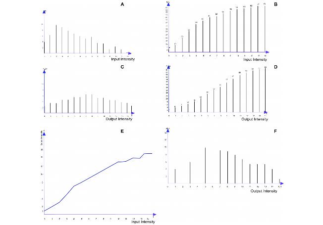
The transformation function is obtained by choosing g for each f, such that if g > f, then Pd(g) > P(f). The transformation function is then applied to the input image to produce an output image by remapping the pixel intensities. The objective is to find a transformed digital picture of a given picture, such that the sum of absolute errors between the intensity level histogram of the transformed picture and that of a reference picture is minimized. Refer to Figure 1.
Figure 1. Histograms and cumulative histograms: (A) histogram of 8x8 pixel image; (B) cumulative histogram derived from (A); (C) desired histogram of the same 8x8 pixel image; (D) cumulative histogram derived from (C); (E) gray scale transformation function that approximately transforms the histogram (A) to desired histogram (C); (F) histogram of gray-scale-transformed image obtained by applying the transformation function in (E) to the image with the histogram shown in (A).
|
|
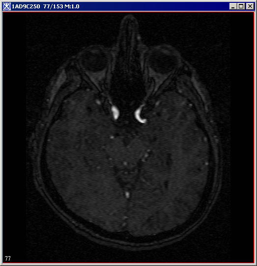
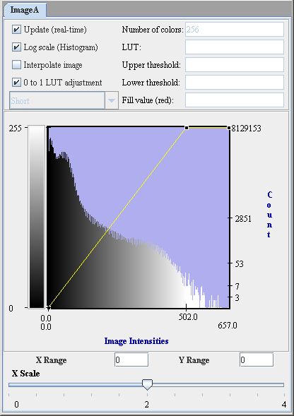
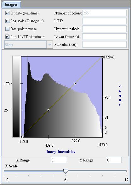
Figure 2. The input image and its histogram p(f)
|
|
|
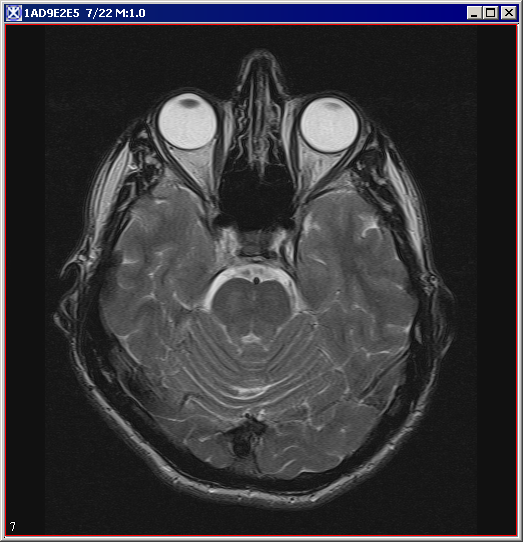
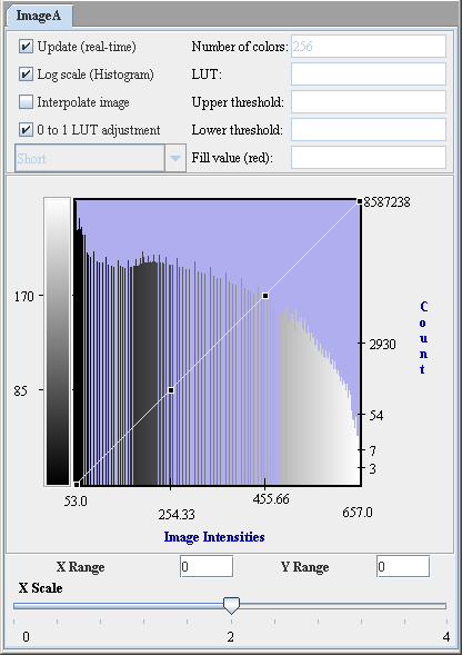
Figure 3. The specified image and its histogram pd(g)
|
|
|
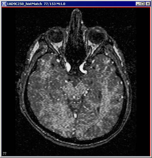
Figure 4. The result image and its histogram
|
|
|
References
Rafael C. Gonzalez and Richard E. Woods. Digital Image Processing. Addison-Wesley Publishing Company, 1992, pp. 173-182
Jae S. Lim. Two-Dimensional Signal and Image Processing. Prentice-Hall, Inc., 1990, pp. 453-459
Image types
You can apply this algorithm to both color and black-and-white images, as well as 2D and 3D images.
Applying the Histogram Matching algorithm
To use this algorithm, do the following:
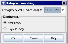
- Select Algorithms > Histogram Tools > Histogram Matching in the main MIPAV window. The Histogram Matching dialog box (Figure 5) appears.
- Complete the information in the dialog box.
- Click OK. The algorithm begins to run, and a progress bar appears momentarily with the status. When the algorithm finishes running, the progress bar disappears, and the results appear in a separate image window.
Figure 5. Histogram Matching dialog box
|
Histogram match <File name> to
|
Select the specified image pd(g) from the list box
|
|
|
New image
|
Shows the results of the algorithm in a new image window
|
|
Replace image
|
Shows the results of the algorithm in the same image window
|
|
OK
|
Applies the algorithm according to the specifications in this dialog box.
|
|
Cancel
|
Disregards any changes that you made in the dialog box and closes this dialog box.
|
|
Help
|
Displays online help for this dialog box.
|


