Filters (Spatial): Regularized Isotropic (Nonlinear) Diffusion and Filters (Spatial): Slice Averaging: Difference between pages
(Difference between pages)
Jump to navigation
Jump to search
m (1 revision imported) |
MIPAV>Olga Vovk mNo edit summary |
||
| Line 1: | Line 1: | ||
''This algorithm provides a way of reducing image noise by summing together a set of noisy images and dividing the sum by the number of images. The algorithm assumes that the noise in the images is uncorrelated and has zero average value.'' | |||
------ | |||
== | {| width="90%" border="1" frame="hsides" frame="hsides" | ||
|- | |||
| width="9%" valign="top" | | |||
[[Image:noteicon.gif]] | |||
| width="81%" bgcolor="#B0E0E6" | | |||
[http://mipav.cit.nih.gov/documentation/HTML Algorithms/FiltersSpatialSliceAveraging.html For more information about the algorithm, refer to the MIPAV web site: {http://mipav.cit.nih.gov/documentation/HTML Algorithms/FiltersSpatialSliceAveraging.html}. ] | |||
|} | |||
<br /> | |||
== Image types == | == Image types == | ||
You can apply this algorithm to all data types | You can apply this algorithm to all image data types and to 2D, 2.5D, and 3D images. | ||
== Applying | == Applying the Slice Averaging algorithm == | ||
To run this algorithm, complete the following steps: | To run this algorithm, complete the following steps: | ||
# Select Algorithms > Filter > | # Open an image. | ||
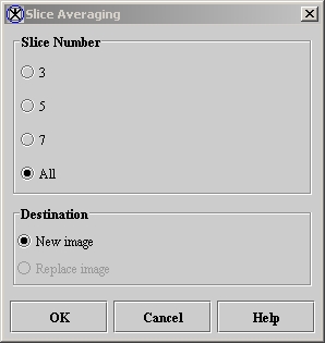
# Select Algorithms > Filter (spatial) > Slice Averaging. The Slice Averaging dialog box (Figure 1) opens. | |||
<div> | |||
{| border="1" cellpadding="5" | {| border="1" cellpadding="5" | ||
|+ <div>'''Figure 1. | |+ <div>'''Figure 1. Slice Averaging dialog box''' </div> | ||
|- | |- | ||
| | | | ||
<div>''' | <div>'''3''' </div> | ||
| | | | ||
<div> | <div>Averages 3 slices in the dataset and creates a 3D image. </div> | ||
| rowspan=" | | rowspan="7" colspan="1" | | ||
<div><div><center>[[Image: | <div><div><center>[[Image:dialogboxSliceAveraging.jpg]]</center></div> </div> | ||
|- | |- | ||
| | | | ||
<div>''' | <div>'''5''' </div> | ||
| | | | ||
<div> | <div>Averages 5 slices in the dataset and creates a 3D image. </div> | ||
|- | |- | ||
| | | | ||
<div>''' | <div>'''7''' </div> | ||
| | | | ||
<div> | <div>Averages 7 slices in the dataset and creates a 3D image. </div> | ||
|- | |- | ||
| | | | ||
<div>''' | <div>'''All''' </div> | ||
| | | | ||
<div> | <div>Averages all of the slices in the dataset and creates a 2D image (default choice). </div> | ||
|- | |||
| | |||
<div>'''New image''' </div> | |||
| | |||
<div>Shows the results of the algorithm in a new image window (default choice). </div> | |||
|- | |||
| | |||
<div>'''Replace image''' </div> | |||
| | |||
<div>Replaces the current active image with the newly calculated <br />image. </div> | |||
|- | |- | ||
| | | | ||
<div>'''OK''' </div> | <div>'''OK''' </div> | ||
| | |||
<div>Applies the algorithm according to the specifications in this dialog box. </div> | <div>Applies the algorithm according to the specifications in this dialog box. </div> | ||
|- | |- | ||
| Line 66: | Line 76: | ||
|} | |} | ||
</div> | |||
# Complete the information in the dialog box. | |||
# Click OK. | |||
; The algorithms begins to run, and a pop-up window appears with the status. The following messages appear: "Averaging data" and "Importing average data." | |||
; When the algorithm finishes running, the pop-up window closes, and the results appear either in a new window or replace the image in which the algorithm was applied. | |||
[[Category:Help]] | [[Category:Help]] | ||
[[Category:Help:Algorithms]] | [[Category:Help:Algorithms]] | ||
Revision as of 18:43, 27 July 2012
This algorithm provides a way of reducing image noise by summing together a set of noisy images and dividing the sum by the number of images. The algorithm assumes that the noise in the images is uncorrelated and has zero average value.
Image types
You can apply this algorithm to all image data types and to 2D, 2.5D, and 3D images.
Applying the Slice Averaging algorithm
To run this algorithm, complete the following steps:
- Open an image.
- Select Algorithms > Filter (spatial) > Slice Averaging. The Slice Averaging dialog box (Figure 1) opens.
|
3
|
Averages 3 slices in the dataset and creates a 3D image.
|
|
|
5
|
Averages 5 slices in the dataset and creates a 3D image.
| |
|
7
|
Averages 7 slices in the dataset and creates a 3D image.
| |
|
All
|
Averages all of the slices in the dataset and creates a 2D image (default choice).
| |
|
New image
|
Shows the results of the algorithm in a new image window (default choice).
| |
|
Replace image
|
Replaces the current active image with the newly calculated
image. | |
|
OK
|
Applies the algorithm according to the specifications in this dialog box.
| |
|
Cancel
|
Disregards any changes that you made in this dialog box and closes the dialog box.
| |
|
Help
|
Displays online help for this dialog box.
| |
- Complete the information in the dialog box.
- Click OK.
- The algorithms begins to run, and a pop-up window appears with the status. The following messages appear
- "Averaging data" and "Importing average data."
- When the algorithm finishes running, the pop-up window closes, and the results appear either in a new window or replace the image in which the algorithm was applied.
