Filters (Spatial): Mean and Filters (Spatial): Mode: Difference between pages
m (1 revision imported) |
MIPAV>Olgavovk mNo edit summary |
||
| Line 1: | Line 1: | ||
Mode filtering is a nonlinear spatial filtering technique that replaces a target pixel with the mode of neighboring pixels. The ''mode'' of a set of values is the value that occurs most frequently within the set. If all values are unique-that is, all numbers occur only once in the set-the value of the target pixel stays the same. Mode filtering is similar in philosophy to median filtering. | |||
Mode filtering is currently thought to be useful in filtering a segmented image to eliminate small clusters of pixels labeled one value that are completely within a large cluster of pixels of a different value. Mode filtering is currently being investigated in improving a C-means classification of brain images, which were first segmented using the brain extraction tool (BET). Mode filtering can be applied to grayscale images to remove some noise; however, a 3 x 3 x 3 cube kernel significantly blurs the image. | |||
=== Background === | === Background === | ||
When you apply the Mode algorithm, MIPAV identifies the target pixel and collects the values of the surrounding neighborhood. Next, it arranges the values of the target and neighborhood pixels in a list and sorts them. The value of the target pixel is replaced with the mode of the numbers in the list. Determining the mode of a sorted list of numbers is done in a single pass through the list by incrementing a count variable each time adjacent values are the same and maintaining the maximum count along with the corresponding value. | |||
Neighborhood pixels are determined by the shape and size of the kernel. (The selection of pixels using the kernel is sometimes referred to as the ''sliding window approach''.) The most common kernel shapes are the square and cross. | |||
Square-shaped kernels are defined as all pixels in the ''k''(''k'') region surrounding the target pixel, where k refers to the window size. Cross-shaped kernels are defined as the central row and column of the ''k''(''k'') region. | |||
The kernel is usually centered on the target pixel and is symmetrical; pixels chosen are symmetrically located about the target pixel. Thus, pixels on opposite sides are equally weighted. The kernel varies in size, although commonly a square kernel can range from 3 to 11 pixels per side. Other kernel shapes and sizes could be selected, but choosing the region of pixels to include always involves juggling the elimination of noise and increasing fuzziness and posterization of an image. | |||
Pixel values are sorted in increasing order. Any sorting method is acceptable, although, because the number of pixels can be large, a fast- sorting algorithms is preferable. The best sorting algorithm is one that can efficiently accommodate both small and large lists. Generally, when considering the number of items to sort, the numbers can range from 5 (in a 3 x 3 cross) to 121 (in an 11 x 11 square). This algorithm implements the Shell-sort because it operates very efficiently for the sizes of the lists expected. | |||
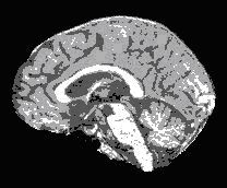
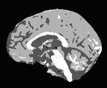
The left image in Figure 1 shows a segmented image that results after applying the C-means classification algorithm to a brain image produced with the brain extraction tool. The image on the right shows the result of applying the Mode filtering algorithm with a 3 x 3 x 3 local neighborhood to the image on the left. Clearly, the image on the right has fewer small isolated classes than the image on the left. | |||
<div> | <div> | ||
{| border="1" cellpadding="5" | {| border="1" cellpadding="5" | ||
|+ <div>'''Figure 1. | |+ <div>'''Figure 1. Examples of (A) a segmented image and (B) the results of applying the Mode algorithm to the image''' </div> | ||
|- | |- | ||
| | | | ||
<div><div><center>[[Image: | <div><div><center>[[Image:exampleMode1.jpg]]</center></div> </div> | ||
| | |||
<div><div><center>[[Image:exampleMode2.jpg]]</center></div> </div> | |||
|} | |} | ||
</div> | </div> | ||
The Mode algorithm processes all pixels in the input image. The algorithm uses a symmetric neighborhood definition around the target pixel, resulting in border pixels, which require special processing. Border pixels correspond to those pixels where the neighborhood of a target pixel is incomplete. Incomplete neighborhoods occur: | |||
* ''In-plane''-In the corners of the image plane | |||
* ''Through-plane''-On the first and last (few) image planes | |||
In-plane border pixels are not filtered and the value assigned to the output pixel is simply the corresponding input value. Through-plane border pixels are filtered by duplicating the values of corresponding pixels on the target pixel plane. | |||
==== Image types ==== | ==== Image types ==== | ||
You can apply this algorithm | You can apply this algorithm to 2D, 2.5D, and 3D images. Since the algorithm counts the number of pixels with the same value, it only allows the following list of data types. | ||
* BYTE and UBBYTE | |||
* SHORT and USHORT | |||
* INTEGER and UINTEGER | |||
==== | ==== Notes ==== | ||
The resulting image is, by default, the same type as the input image. | |||
==== References ==== | ==== References ==== | ||
This algorithm was developed by members of the MIPAV team. Mode filtering is similar to median filtering, and to our knowledge there is not a significant amount of literature about the topic. | |||
=== Applying the | === Applying the Mode algorithm === | ||
To run this algorithm, complete the following steps: | To run this algorithm, complete the following steps: | ||
# Open an image | # Open an image. | ||
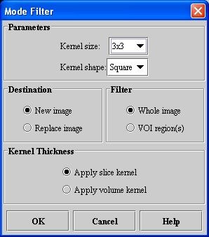
# Select Algorithms > | # Select Algorithms > Filters (Spatial) > Mode. The Mode Filter dialog box ([FiltersSpatialMode.html#wp1006320 Figure 35]) opens. | ||
# Complete the | # Complete the fields in the dialog box. | ||
# Click OK. | # Click OK when complete. The algorithm begins to run. | ||
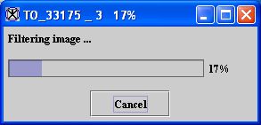
; | ; A pop-up window appears with the status. | ||
<div> | <div> | ||
{| border="1" cellpadding="5" | {| border="1" cellpadding="5" | ||
|+ | |+ | ||
|- | |- | ||
| | | | ||
<div> | <div><div><center>[[Image:messageModeFiltering.jpg]]</center></div> </div> | ||
| | |} | ||
<div> | |||
| | </div> | ||
<div> | |||
; When the algorithm finishes running, the pop-up window closes. | |||
; Depending on whether New image or Replace image was selected, results appear in a new window or replace the image to which the algorithm was applied. | |||
<div> | |||
{| border="1" cellpadding="5" | |||
|+ <div>'''Figure 2. Mode Filter dialog box ''' </div> | |||
|- | |- | ||
| | | | ||
<div>''' | <div>'''Kernel size''' </div> | ||
| | | | ||
<div> | <div>Specifies the size of the local neighborhood when performing mode filtering. A ''k'' x ''k'' region selects a neighborhood that extends in all directions by (''k'' - 1)/2 placing the target pixel in the center of the kernel. Kernels for 2D images are odd valued and include 3 x 3, 5 x 5, 7 x 7, and so on. </div> | ||
| rowspan="4" colspan="1" | | |||
<div><div><center>[[Image:dialogboxModeFilter.jpg]]</center></div> </div> | |||
|- | |- | ||
| | | | ||
<div>''' | <div>'''Kernel shape''' </div> | ||
| | | | ||
<div> | <div>Selects which pixels in the kernel size box are included as a part of the mode's neighborhood. </div> | ||
|- | |- | ||
| | | | ||
<div>'''New image''' </div> | <div>'''New image''' </div> | ||
| | | | ||
<div> | <div>Indicates where the results of the algorithm appear. If you select this option, the results appear in a new image window. </div> | ||
|- | |- | ||
| | | | ||
<div>'''Replace image''' </div> | <div>'''Replace image''' </div> | ||
| | | | ||
<div> | <div>Indicates where the results of the algorithm appear. If you select this option, the results replace the current active image. </div> | ||
|- | |- | ||
| | | | ||
<div>'''Whole image''' </div> | <div>'''Whole image''' </div> | ||
| | | rowspan="1" colspan="2" | | ||
<div>Applies the algorithm to the whole image. </div> | <div>Applies the algorithm to the whole image. </div> | ||
|- | |- | ||
| | | | ||
<div>'''VOI | <div>'''VOI region(s)''' </div> | ||
| rowspan="1" colspan="2" | | | rowspan="1" colspan="2" | | ||
<div>Applies the algorithm to the volumes (regions) delineated by the VOIs. </div> | <div>Applies the algorithm to the volumes (regions) delineated by the VOIs. </div> | ||
| Line 134: | Line 118: | ||
<div>'''Apply slice kernel''' </div> | <div>'''Apply slice kernel''' </div> | ||
| rowspan="1" colspan="2" | | | rowspan="1" colspan="2" | | ||
<div> | <div>Filters each slice of the image independently of other slices, finding neighboring pixels from the slice. </div> | ||
|- | |- | ||
| | | | ||
<div>'''Apply volume kernel''' </div> | <div>'''Apply volume kernel''' </div> | ||
| rowspan="1" colspan="2" | | | rowspan="1" colspan="2" | | ||
<div> | <div>Gathers pixel values from the slice as well as from neighboring slices. </div> | ||
|- | |- | ||
| | | | ||
<div>'''OK''' </div> | <div>'''OK''' </div> | ||
| rowspan="1" colspan="2" | | | rowspan="1" colspan="2" | | ||
<div>Applies the | <div>Applies the Mode filtering algorithm according to the specifications in this dialog box. </div> | ||
|- | |- | ||
| | | | ||
| Line 156: | Line 140: | ||
<div>Displays online help for this dialog box. </div> | <div>Displays online help for this dialog box. </div> | ||
|} | |} | ||
[[Category:Help]] | [[Category:Help]] | ||
[[Category:Help:Algorithms]] | [[Category:Help:Algorithms]] | ||
Revision as of 18:26, 18 May 2012
Mode filtering is a nonlinear spatial filtering technique that replaces a target pixel with the mode of neighboring pixels. The mode of a set of values is the value that occurs most frequently within the set. If all values are unique-that is, all numbers occur only once in the set-the value of the target pixel stays the same. Mode filtering is similar in philosophy to median filtering.
Mode filtering is currently thought to be useful in filtering a segmented image to eliminate small clusters of pixels labeled one value that are completely within a large cluster of pixels of a different value. Mode filtering is currently being investigated in improving a C-means classification of brain images, which were first segmented using the brain extraction tool (BET). Mode filtering can be applied to grayscale images to remove some noise; however, a 3 x 3 x 3 cube kernel significantly blurs the image.
Background
When you apply the Mode algorithm, MIPAV identifies the target pixel and collects the values of the surrounding neighborhood. Next, it arranges the values of the target and neighborhood pixels in a list and sorts them. The value of the target pixel is replaced with the mode of the numbers in the list. Determining the mode of a sorted list of numbers is done in a single pass through the list by incrementing a count variable each time adjacent values are the same and maintaining the maximum count along with the corresponding value.
Neighborhood pixels are determined by the shape and size of the kernel. (The selection of pixels using the kernel is sometimes referred to as the sliding window approach.) The most common kernel shapes are the square and cross.
Square-shaped kernels are defined as all pixels in the k(k) region surrounding the target pixel, where k refers to the window size. Cross-shaped kernels are defined as the central row and column of the k(k) region.
The kernel is usually centered on the target pixel and is symmetrical; pixels chosen are symmetrically located about the target pixel. Thus, pixels on opposite sides are equally weighted. The kernel varies in size, although commonly a square kernel can range from 3 to 11 pixels per side. Other kernel shapes and sizes could be selected, but choosing the region of pixels to include always involves juggling the elimination of noise and increasing fuzziness and posterization of an image.
Pixel values are sorted in increasing order. Any sorting method is acceptable, although, because the number of pixels can be large, a fast- sorting algorithms is preferable. The best sorting algorithm is one that can efficiently accommodate both small and large lists. Generally, when considering the number of items to sort, the numbers can range from 5 (in a 3 x 3 cross) to 121 (in an 11 x 11 square). This algorithm implements the Shell-sort because it operates very efficiently for the sizes of the lists expected.
The left image in Figure 1 shows a segmented image that results after applying the C-means classification algorithm to a brain image produced with the brain extraction tool. The image on the right shows the result of applying the Mode filtering algorithm with a 3 x 3 x 3 local neighborhood to the image on the left. Clearly, the image on the right has fewer small isolated classes than the image on the left.
The Mode algorithm processes all pixels in the input image. The algorithm uses a symmetric neighborhood definition around the target pixel, resulting in border pixels, which require special processing. Border pixels correspond to those pixels where the neighborhood of a target pixel is incomplete. Incomplete neighborhoods occur:
- In-plane-In the corners of the image plane
- Through-plane-On the first and last (few) image planes
In-plane border pixels are not filtered and the value assigned to the output pixel is simply the corresponding input value. Through-plane border pixels are filtered by duplicating the values of corresponding pixels on the target pixel plane.
Image types
You can apply this algorithm to 2D, 2.5D, and 3D images. Since the algorithm counts the number of pixels with the same value, it only allows the following list of data types.
- BYTE and UBBYTE
- SHORT and USHORT
- INTEGER and UINTEGER
Notes
The resulting image is, by default, the same type as the input image.
References
This algorithm was developed by members of the MIPAV team. Mode filtering is similar to median filtering, and to our knowledge there is not a significant amount of literature about the topic.
Applying the Mode algorithm
To run this algorithm, complete the following steps:
- Open an image.
- Select Algorithms > Filters (Spatial) > Mode. The Mode Filter dialog box ([FiltersSpatialMode.html#wp1006320 Figure 35]) opens.
- Complete the fields in the dialog box.
- Click OK when complete. The algorithm begins to run.
- A pop-up window appears with the status.
- When the algorithm finishes running, the pop-up window closes.
- Depending on whether New image or Replace image was selected, results appear in a new window or replace the image to which the algorithm was applied.
|
Kernel size
|
Specifies the size of the local neighborhood when performing mode filtering. A k x k region selects a neighborhood that extends in all directions by (k - 1)/2 placing the target pixel in the center of the kernel. Kernels for 2D images are odd valued and include 3 x 3, 5 x 5, 7 x 7, and so on.
|
|
|
Kernel shape
|
Selects which pixels in the kernel size box are included as a part of the mode's neighborhood.
| |
|
New image
|
Indicates where the results of the algorithm appear. If you select this option, the results appear in a new image window.
| |
|
Replace image
|
Indicates where the results of the algorithm appear. If you select this option, the results replace the current active image.
| |
|
Whole image
|
Applies the algorithm to the whole image.
| |
|
VOI region(s)
|
Applies the algorithm to the volumes (regions) delineated by the VOIs.
| |
|
Apply slice kernel
|
Filters each slice of the image independently of other slices, finding neighboring pixels from the slice.
| |
|
Apply volume kernel
|
Gathers pixel values from the slice as well as from neighboring slices.
| |
|
OK
|
Applies the Mode filtering algorithm according to the specifications in this dialog box.
| |
|
Cancel
|
Disregards any changes that you made in this dialog box and closes the dialog box.
| |
|
Help
|
Displays online help for this dialog box.
| |


