This page contains instructions on how to perform MRI prostate segmentation and surface reconstruction in MIPAV. The algorithm facilities the validation of multi-parametric MRI with histopathology slides from radical prostatectomy specimens and targeted biopsy specimens. It employs the technique that combines image processing and computer aided design to construct a high resolution 3D prostate surface from MRI images in three orthogonal views with non-isotropic voxel resolution.
The algorithm outline is shown below, refer to (Applying the algorithm.
Image types
The algorithm could be applied to the following image types (TBD). In order to use the segmentation tool, the image dataset must contain 3 orthogonal images centered at prostate center, similar to ones in the sample image dataset available for download via this link.
Sample image dataset
We encourage you to test the algorithm on the prostate images provided in the sample image dataset. The sample image dataset provided by NCI can be downloaded using this link. The data included are orthogonal MR images obtained from a 3.0 T whole-body MRI system (Achieva, Philips Healthcare).
T2-weighted MR images of the entire prostate were obtained in three orthogonal planes (sagittal, axial and coronal) using the following settings:
- Scan resolution of 0.2734x0.2734x3.0 cubic millimeters,
- Field of view - 140 mm,
- Image slice dimension 512x512.
The center of the prostate is the focal point for the MRI scan. To reduce the scan time, a lower refocusing pulse of 100 degrees was used for sagittal and coronal images, which alters the contrast on these images compared to the axial images.
Applying the algorithm
Applying the algorithm involves the following major steps:
- Opening 3 orthogonal images and delineating VOIs eitehr manually or using VOIs from the the test image dataset
- Prostate segmentation using Automatic B-Spline Registration algorithm
- Prostate surface reconstruction
- 3D Visualization and STL surface generation
Opening images and delineating VOIs
If you are working with DICOM images, convert DICOM images into MIPAV XML format, first. In order to do that,
- Open a DICOM image. Refer to Working with DICOM Images for more information.
- Convert a DICOM image dataset into MIPAV XML format. Use File > Save Image As menu.
Naming conventions: When you convert a DICOM image to a MIPAV XML image, we advise you to use the following file names: image_ax_83.xml, image_sag_83.xml, image_cor_83.xml. The ax, sag, and cor suffixes are used to specify axial, sagittal, and coronal images correspondingly. These are names used in the the sample image dataset. And these are file names used in this instruction.
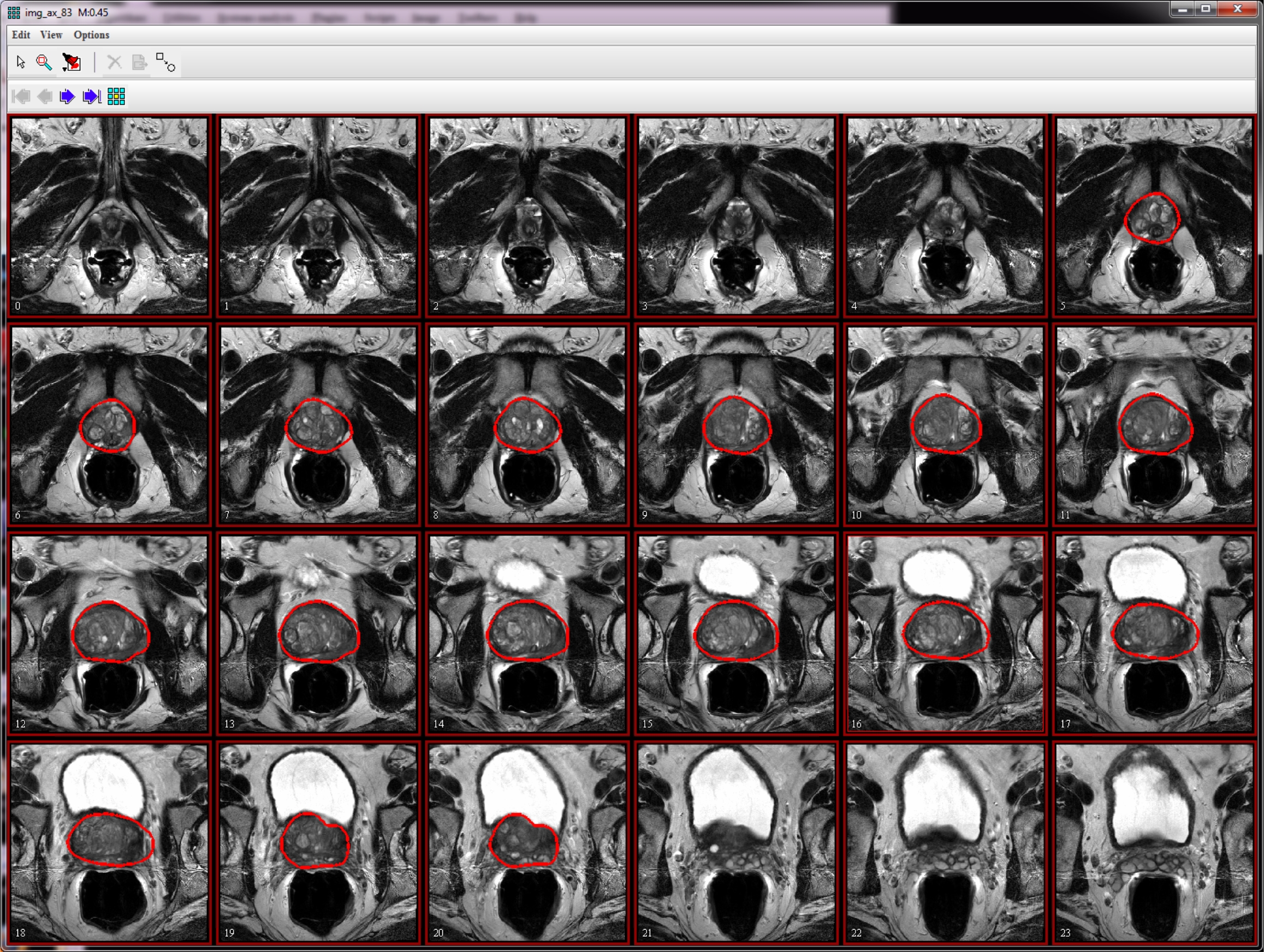
To open an axial image, use File > Open image (A) from disk menu. If you are using the sample image dataset provided, open the img_ax_83.xml file.
To delineate prostate VOIs, use the Polygon/Polyline VOI tool ![]() from the MIPAV toolbar.
from the MIPAV toolbar.
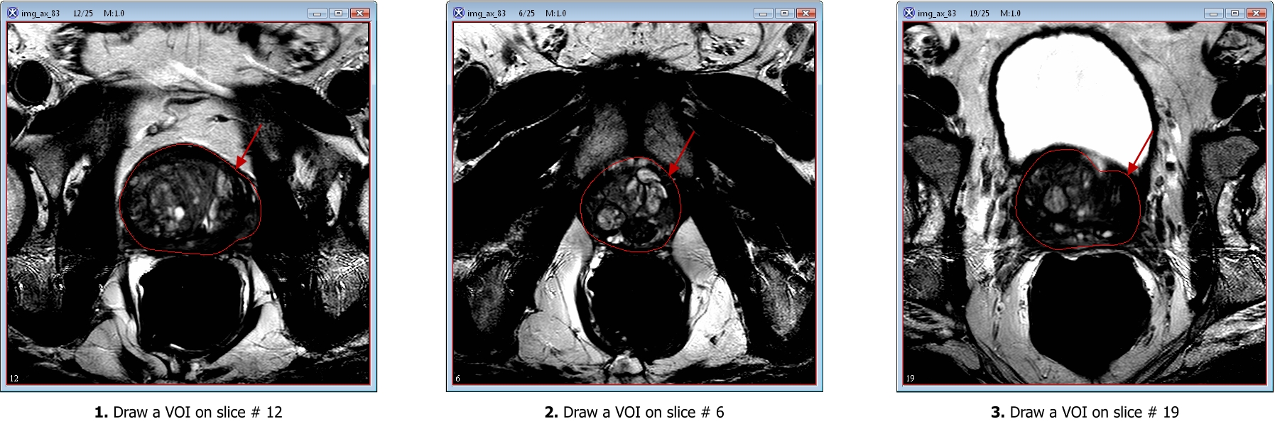
For example, if you work with the sample image dataset:
- Draw the apex VOI, on slice #6 of the img_ax_83.xml file;
- Draw the mid slice VOI, on slice #12;
- Draw the last VOI on the base slice #19.
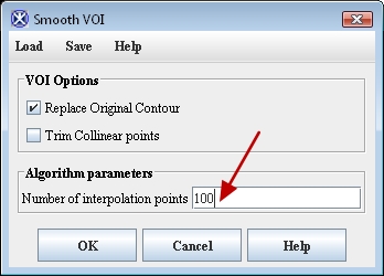
Smoothing VOIs. After delineating VOIs, we need to smooth each VOI. In order to do this, select each VOI and call the Smooth VOI dialog box. The dialog is available from the main MIPAV menu (VOI > Smooth VOI).
In the Smooth VOI dialog box, check the "Replace Original Contour" box, and set "Number of interpolation points" to 100. Click OK. Repeat for all 3 contours.
Sagittal and coronal images. Repeat the same process of delineating and smoothing VOIs for both sagittal and coronal images. In the sample image dataset provided, the saggital image name is img_sag_83 and the coronal image name is img_cor_83. See Naming Conventions.
Example
In the sample image dataset provided, VOIs files are already available for all 3 types of images (axial, saggital and coronal). Under the image dataset directory, one can find 3 orthogonal images and corresponding VOIs:
| Orientation | Image file | VOI file |
|---|---|---|
| axial | img_ax_83.xml | voi_ax_83.xml |
| coronal | img_cor_83.xml | voi_cor_83.xml |
| saggital | img_sag_83.xml | voi_sag_83.xml |
Note: The VOIs from the sample image dataset were drawn by clinical researchers, and verified by radiologist expert at NCI. For experimental purposes, we could recommend performing quick VOIs copying instead of manually drawing all three VOIs for all 3 image files.
To copy VOIs
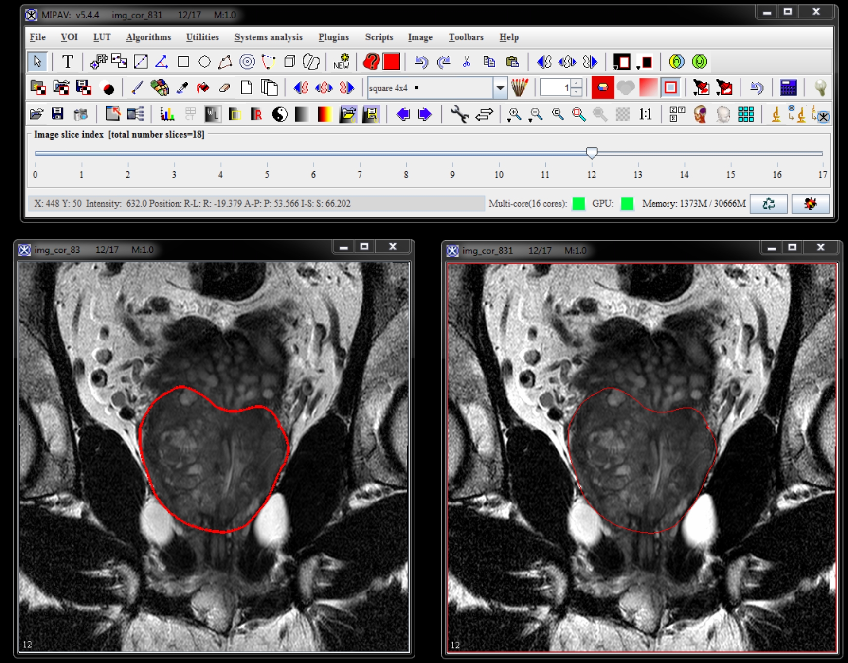
- Open the same image twice, and open the VOIs file for the extra opened image. Let's name the first opened image the source image and the second opened image the extra image.
- From the MIPAV toolbar, use the Link Images tool
 to link the two images. Please, make sure to open the same image slice on each image, i.e. #12, before linking the images.
 - Slide through the two images in parallel mode.
- Consequently open slices 6, 12, and 19 and make sure to copy 3 corresponding VOIs from the extra image to the source image.
- After finishing copying the three VOIs, unlink the two images.
- Close the extra image.
- Use the Smooth VOI dialog box options to smooth the VOIs contours to 100 points.
- Repeat the same procedure for all three, axial, sagittal and coronal images.
Prostate segmentation
We use the semi-automatic segmentation dialog to segment the MRI prostate image. Before proceeding, please, make sure you open 3 orthogonal prostate images with VOIs - img_ax_83.xml and voi_ax_83.xml, img_sag_83.xml and voi_ax_sag.xml, and img_cor_83.xml and voi_cor_83.xml.
Automatic B-Spline registration guided MRI prostate segmentation
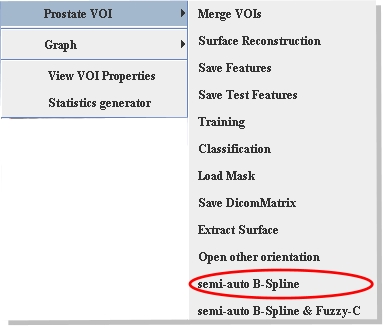
- From the MIPAV main menu, use the VOI->Prostate VOI->semi-auto BSpline menu to run the Prostate Segmentation dialog.
- The dialog box appears.
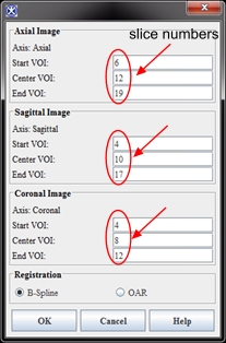
Note that the drawn VOIs slice numbers are automatically populated in the dialog box.
- In the Prostate Segmentation dialog, the Registration B-Spline radio check box is selected by default.
- Click OK to start the concurrent automatic prostate segmentation procedure.
- The algorithm begins to run and segmentation results appear on the screen and in the console window. For the B-Spline registration guided MRI prostate segmentation, the whole procedure takes 2 minutes to finish the segmentation, see MIPAV Console window.
For each named VOIs based mask, the console window shows the number of voxels and volume. Created VOIs are used for the surface reconstruction step. Each VOI contour has 100 points.
MIPAV Console window
Axial image VOIs:  number of voxels = 333795  volume = 74871.586 mm^3
Sagittal image VOIs:  number of voxels = 340633  volume = 76405.41 mm^3
Coronal image VOIs:  number of voxels = 320149  volume = 71810.766 mm^3
time elapse = 1  mins  55  sec
Saving VOIs
To save each new segmented VOI, select the VOI first, and then call the Save VOI dialog box.
To avoid confusions save these VOIs separately as _new.xml files. You can consider using the following naming convention for the axial, sagittal, and coronal VOIs respectively: voi_ax_new.xml, voi_sag_new.xml and voi_cor_new.xml
Merging VOIs
To form a cloud points set used for surface reconstruction, we need to merge 3 VOIs (axial, coronal and sagittal) in DICOM space.
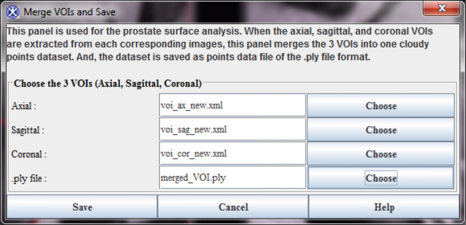
- To merge VOIs, choose the VOI->Prostate VOI->Merge VOIs menu. The Merge VOIs dialog box appears.
- In the dialog box, select 3 saved VOIs files.
- Specify the final point set data file (.ply), which combines 3 VOIs into a single cloud point set. For example, give it the following name "merged_VOI.ply".
- Click Save to save.
Surface reconstruction
We provide a unified dialog to use the Ball-Pivoting and Poisson surface reconstruction algorithms to build the smooth 3D surface with the generated point cloud dataset.
Input - the final point set data file - merged_VOI.ply.
Output - the final surface file -prostate_surface.ply and the coarse surface output file bpt_output.ply.
To run the Surface Reconstruction algorithm:
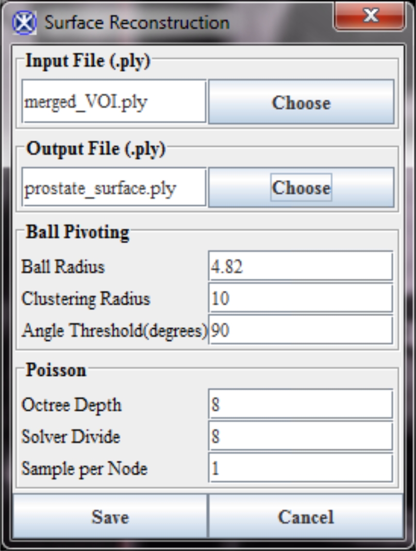
- Open the Surface Reconstruction dialog box, use the VOI->Prostate VOI->Surface Reconstruction menu.
- Use the .ply file (e.g. merged_VOI.ply) as an input.
- In the dialog box, the Ball-pivoting and Poisson parameters are set to defaults which could be modified by the user.
- Click Save to start the surface reconstruction algorithm. The algorithm begins to run. For a could created from 3 100-point VOIs the surface reconstruction algorithm run time is approximately 1 minute.
- The output file is the final surface .ply file. The default file name is "prostate_surface.ply", but it can be changed by the user. To change the file name use the Choose button.
The coarse surface output file
The coarse surface output file is generated after running the Ball-Pivoting algorithm. The surface is constructed with many holes left. The Poisson algorithm takes the coarse surface as an input, and finishes up with a final smoothed prostate surface.
3D Visualization and STL surface generation
After generating the smoothed prostate surface, the MIPAV GPU based 3D visualization software is used to prepare the surface data for 3D printing. The axial image is used to visualize the prostate surface. This is because the apex and base VOIs contours of axial image might be big enough to go beyond the sagittal and coronal image boundary. Thus, the axial image is the best to hold the final generated prostate surface.
Saving an axial image DICOM matrix
MIPAV GPU based Volume Renderer works with DICOM matrix files, therefore we need to save the axial image DICOM matrix. During visualization, the DICOM matrix file is used to transfer the surface points from DICOM space to image space.
In order to save the DICOM matrix:
- Open the axial image, i.e. img_ax_83.xml.
- From MIPAV top menu select VOI->Prostate VOI->Save DicomMatrix.
- By default, a DICOM matrix file is saved under the current axial image directory, i.e. img_ax_83.dicomMatrix.
Note: in MIPAV all axial, sagittal, and coronal VOIs are saved in DICOM space, therefore the final generated prostate surface is also saved in DICOM space.
3D GPU based visualization
See also Volume renderer GPU support listing.
Input - the DICOM matrix file, e.g. img_ax_83.dicomMatrix
Output - STL surface file, e.g.3D printing_Prostate.stl
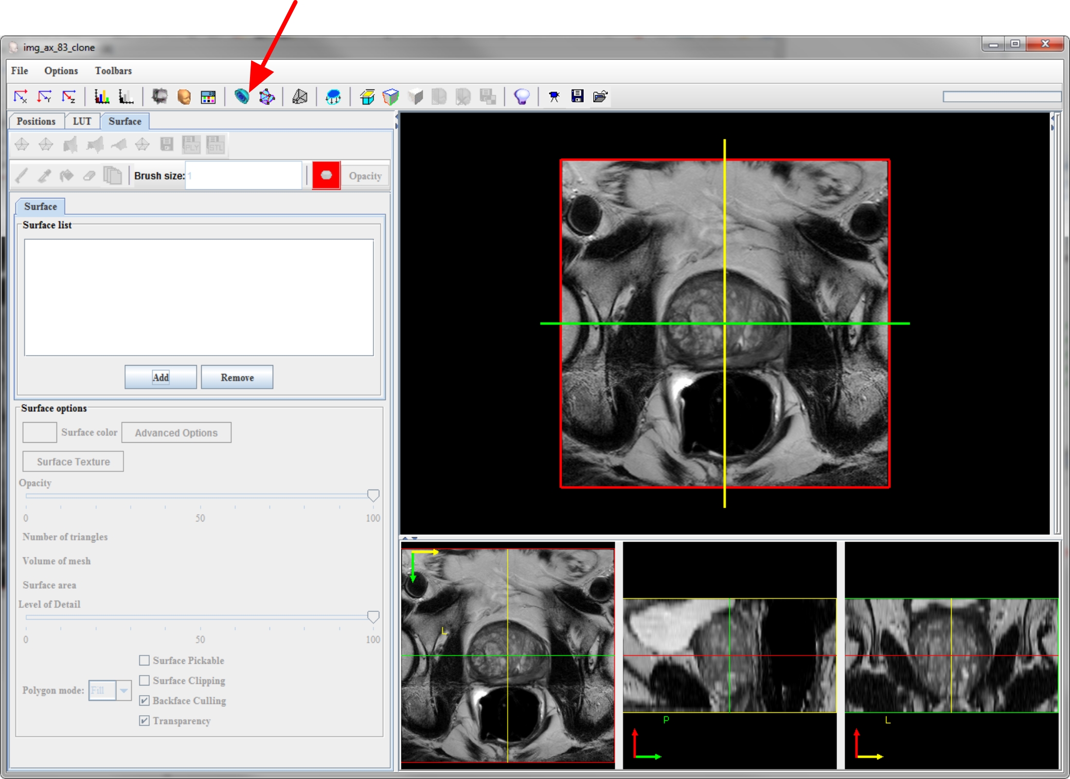
![]() - To run MIPAV GPU Renderer, click the GPU based Volume Renderer icon on MIPAV toolbar. The MIPAV GPU Visualization window appears (see a in the figure below).
- To run MIPAV GPU Renderer, click the GPU based Volume Renderer icon on MIPAV toolbar. The MIPAV GPU Visualization window appears (see a in the figure below).
- In the MIPAV GPU Visualization window, click on the Surface icon
 to open the Surface Reconstruction panel (see b in the figure below).
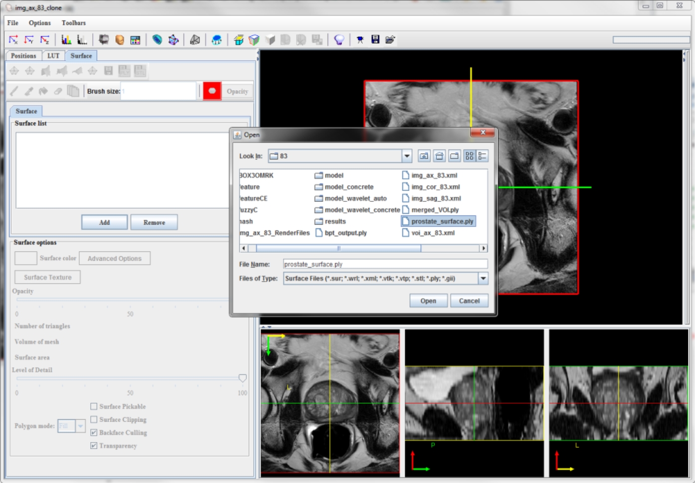
 - In the Surface Reconstruction panel, click Add to add the prostate surface, and specify the prostate surface file, e.g. prostate_surface.ply, as shown below (see c in the figure below).
- In the dialog box that appears, specify the saved DICOM matrix file (e.g. img_ax_83.dicomMatrix) and click Open.
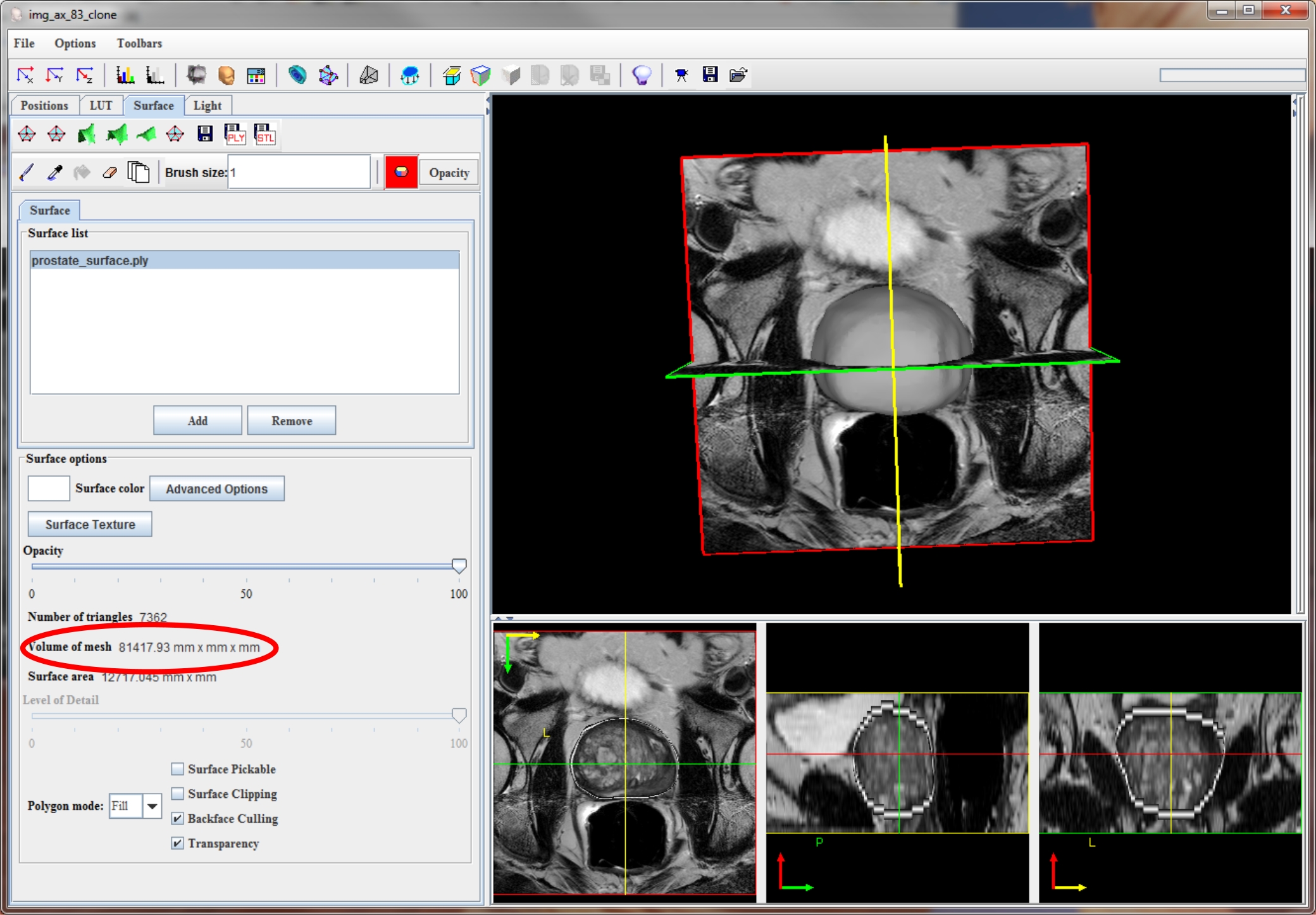
- The smoothed prostate surface appears.
- Inside the Surface panel, Volume of mesh shows the 3D surface volume (see d in the figure below).
 |
 |
 |
 |
Surface decimation and STL surface file generation
The uploaded surface contains 7362 triangles. For the final 3D prostate mold printing, this number is too big. We need to decimate the surface to a smaller number of triangles, and make the triangle meshes printable with Solidworks 3D CAD software.
To decimate the surface
- In the surface panel, click Decimate icon.
- The Level of Detail slider appears.
- Drag the slider from 100 to around 40. You will find the surface triangle meshes being reduced instantly. For example, the number of triangles info shown in figure below was reduced by 2502 triangles.
- To save the decimated surface STL file format,click Save.
- The STL surface file (e.g. 3D printing_Prostate.stl) is used by Solidworks 3D CAD software to generate the 3D prostate mold.
3D Printing
The final prostate 3D surface STL file is imported into Solidworks 3D CAD software to generate the mold.
- The process starts with a solid rectangular block with parallel cutting slots space 6 mm apart.
- It subtracts the prostate surface from the center of the rectangular block, and the resulting mold was split perpendicular to the cutting slots to create two-halves.
- The cutting slots in the mold are parallel to the slices of axial MRI images. That allows the final cutting specimen block slides to correlate 1 to 1 with corresponding axial MRI image slices.
- A Dimension Elite 3D printer was used to fabricate the 3D mold.
Segmentation performance evaluation
To quantitatively evaluate the performance of the semi-automatic segmentation algorithm, comparison based on VOIs binary mask, VOIs volume and 3D prostate surface volume are conducted.
VOIs binary mask method generates the binary mask from VOIs. Then it compares the overlapped region with false negative (FN), false positive (FP), and true positive (TP) volume fractions.
The VOI binary masks use the expert manual segmentation as the established truth. Truth Positive (TP) reflects the majority overlapped region between the semi-automatic and manual segmentation.
For volumetric measure, the VOIs volume is computed by multiplying the total VOI pixels with a single voxel volume. The 3D surface volume is calculated from the binary surface volumetric mask by multiplying the total surface volumetric voxels with a single voxel volume.
Segmentation quality evaluation
The expert drawn VOIs files are provided in the sample image dataset. To compare the image wise segmentation quality, we simply add the expert drawn VOI file into the segmented result image.