Filters (Spatial) Anisotropic Diffusion and Filters (Spatial) Laplacian: Difference between pages
MIPAV>Olga Vovk mNo edit summary |
MIPAV>Olga Vovk No edit summary |
||
| Line 1: | Line 1: | ||
''Edge detection'' is the identification of meaningful discontinuities in gray level or color images. Edges are formed between two regions that have differing intensity values. This algorithm calculates the laplacian of an image (or VOI of the image) using the second derivatives (''Gxx'', ''Gyy'', and ''Gzz'' [3D]) of the Gaussian function at a user-defined scale sigma [standard deviation (SD)] and convolving it with image. The convolution of the second derivatives of the Gaussian with an image is a robust method of extracting edge information. By varying the SD, a scale-space of edges can easily be constructed. | |||
=== | === Background === | ||
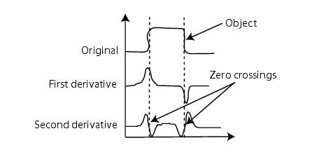
Figure 1 shows the 1D signal of an object. The first derivative of the object is shown next. Last, the Laplacian (defined later) is shown. Note that the zero-crossing of the second derivative corresponds to the edges of the object. | |||
Figure 1 | |||
<div> | |||
{| border="1" cellpadding="5" | {| border="1" cellpadding="5" | ||
|+ <div>'''Figure 1. | |+ <div>'''Figure 1. Edge detection using laplacian operators''' </div> | ||
|- | |- | ||
| | | | ||
<div><div | <div><div align="left">[[Image:LaplacianGrid5.jpg]]</div> </div> | ||
|} | |} | ||
</div> | </div> | ||
= | The laplacian function is defined as:'''' | ||
<math> | |||
\triangledown^2G(x,y) = \frac {\partial^2G}{\partial x^2} + \frac {\partial^2G}{\partial y^2} | |||
</math> | |||
An efficient method of calculating the laplacian is to analytically calculate the second derivatives of Gaussian and convolve the sum with the image. The equation for this calculation follows: | |||
<div align="left">[[Image:FiltersSpatialLaplacian5.jpg]]</div> <div> | |||
{| border="1" cellpadding="5" | {| border="1" cellpadding="5" | ||
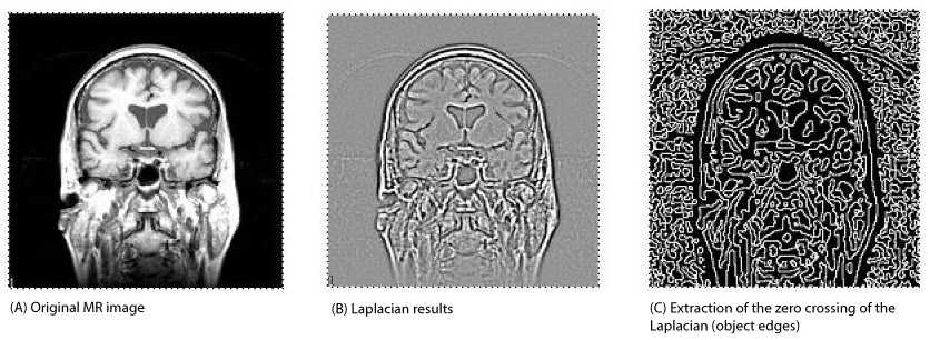
|+ | |+ <div>'''Figure 2. (A) Original MR image; (B) laplacian results; and (C) extraction of the zero crossing of the laplacian (object edges)''' </div> | ||
|- | |- | ||
| | | | ||
<div><div | <div><div><center>[[Image:exampleLaplacianProcessing.jpg]]</center></div> </div> | ||
|} | |} | ||
</div><div><br /> </div> | |||
==== Image types ==== | ==== Image types ==== | ||
You can apply this algorithm | You can apply this algorithm to all image data types except complex and to 2D, 2.5D, and 3D images. | ||
==== Special notes ==== | |||
The resulting image is, by default, a float type image. | |||
To achieve 2.5D blurring (each slice of the volume is processed independently) of a 3D dataset, select Process each slice independently (2.5D) in the Laplacian dialog box (Figure 3). | |||
==== | ==== References ==== | ||
Refer to the | Refer to the following references for more information about this algorithm: | ||
Tony Lindeberg, "Linear Scale-Space I: Basic Theory," ''Geometry-Driven Diffusion in Computer Vision'', Bart M. Ter Har Romeney, ed. (Dordrecht, The Netherlands: Kluwer Academic Publishers, 1994), pp. 1-38. | |||
J. J. Koenderink, "The Structure of Images," ''Biol Cybern'' 50:363-370, 1984. | |||
Raphael C. Gonzalez and Richard E. Woods, ''Digital Image Processing'' (Boston: Addison-Wesley, 1992). | |||
=== Applying the Laplacian algorithm === | |||
=== Applying the | |||
To run this algorithm, complete the following steps: | To run this algorithm, complete the following steps: | ||
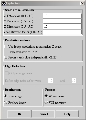
# Select Algorithms > Filter > Laplacian. The Laplacian dialog box opens (Figure 3). | |||
# Complete the fields in the dialog box. | |||
# Select Algorithms > | # When complete, click OK. The algorithm begins to run. | ||
# Complete the | |||
; A pop-up window appears with the status. The following message appears: " | ; A pop-up window appears with the status. The following message appears: "Calculating the Laplacian." | ||
; When the algorithm finishes | ; When the algorithm finishes, the pop-up window closes. Depending on whether you selected New Image or Replace Image, the results either appear in a new window or replace the image to which the algorithm was applied. | ||
<div> | <div>. | ||
{| border="1" cellpadding="5" | {| border="1" cellpadding="5" | ||
|+ <div>'''Figure 3. | |+ <div>'''Figure 3. Laplacian dialog box ''' </div> | ||
|- | |- | ||
| | | | ||
<div>'''X | <div>'''X Dimension''' </div> | ||
| | | | ||
<div> | <div>Specifies the standard deviation (SD) of Gaussian in the ''X'' direction. </div> | ||
| rowspan="6" colspan="1" | | | rowspan="6" colspan="1" | | ||
<div><div><center>[[Image: | <div><div><center>[[Image:dialogboxLaplacian.jpg]]</center></div> </div><div><br /> </div><div><br /> </div> | ||
|- | |||
| | |||
<div>'''Y Dimension''' </div> | |||
| | |||
<div>Specifies the SD of Gaussian in the ''Y'' direction. </div> | |||
|- | |- | ||
| | | | ||
<div>''' | <div>'''Z Dimension''' </div> | ||
| | | | ||
<div> | <div>Specifies the SD of Gaussian in the ''Z'' direction. </div> | ||
|- | |- | ||
| | | | ||
<div>''' | <div>'''Amplification factor''' </div> | ||
| | | | ||
<div> | <div>Applies, by default, the classical laplacian factor of 1.0; values greater than 1.0 and less than 1.2 enable the laplacian to act as a high-pass, or high-boost, filter. </div> | ||
|- | |- | ||
| | | | ||
<div>'''Use image resolutions to normalize Z scale''' </div> | <div>'''Use image resolutions to normalize Z scale''' </div> | ||
| | | | ||
<div>Normalizes the Gaussian to compensate for the difference if the voxel resolution is less | <div>Normalizes the Gaussian to compensate for the difference if the voxel resolution is less than the voxel resolution inplane. </div> | ||
|- | |- | ||
| | | | ||
<div>'''Process each | <div>'''Process each edge independently (2.5D)''' </div> | ||
| | | | ||
<div>Blurs each slice of the dataset independently. </div> | <div>Blurs each slice of the dataset independently. </div> | ||
|- | |- | ||
| | | | ||
<div>''' | <div>'''Output edge image''' </div> | ||
| | | rowspan="1" colspan="2" | | ||
<div> | <div>Produces a binary image that represents the edges defined by the 0 crossings of the laplacian </div> | ||
|- | |- | ||
| | | | ||
<div>''' | <div>'''Threshold edge noise between <_> and <_>''' </div> | ||
| rowspan="1" colspan="2" | | | rowspan="1" colspan="2" | | ||
<div> | <div>Limits the threshold edge noise to the range that you specify between the 0 crossings of the laplacian; the default range is -10 to 10. </div> | ||
|- | |- | ||
| | | | ||
| Line 149: | Line 129: | ||
|- | |- | ||
| | | | ||
<div>'''VOI | <div>'''VOI region(s)''' </div> | ||
| rowspan="1" colspan="2" | | | rowspan="1" colspan="2" | | ||
<div>Applies the algorithm to the volumes (regions) delineated by the VOIs. </div> | <div>Applies the algorithm to the volumes (regions) delineated by the VOIs. </div> | ||
| Line 156: | Line 136: | ||
<div>'''OK''' </div> | <div>'''OK''' </div> | ||
| rowspan="1" colspan="2" | | | rowspan="1" colspan="2" | | ||
<div>Applies the algorithm according to the specifications in this dialog box. </div> | <div>Applies the laplacian algorithm according to the specifications in this dialog box. </div> | ||
|- | |- | ||
| | | | ||
<div>'''Cancel''' </div> | <div>'''Cancel''' </div> | ||
| rowspan="1" colspan="2" | | | rowspan="1" colspan="2" | | ||
<div>Disregards any changes you made in this dialog box and closes the dialog box. </div> | <div>Disregards any changes that you made in this dialog box and closes the dialog box. </div> | ||
|- | |- | ||
| | | | ||
| Line 167: | Line 147: | ||
| rowspan="1" colspan="2" | | | rowspan="1" colspan="2" | | ||
<div>Displays online help for this dialog box. </div> | <div>Displays online help for this dialog box. </div> | ||
|} | |} | ||
== See also: == | |||
**[[Fast Fourier Transformation (FFT)]] | |||
**[[Filters (Spatial): Adaptive Noise Reduction]] | |||
**[[Filters (Frequency)]] | |||
**[[Filters (Spatial): Adaptive Path Smooth]] | |||
**[[Filters (Spatial) Anisotropic Diffusion]] | |||
**[[Filters (Spatial): Coherence-Enhancing Diffusion]] | |||
**[[Filters (Spatial): Gaussian Blur]] | |||
**[[Filters (Spatial): Gradient Magnitude]] | |||
**[[Filters (Spatial): Haralick Texture]] | |||
**[[Filters (Spatial) Laplacian]] | |||
**[[Filters (Spatial): Local Normalization]] | |||
**[[Filters (Spatial): Mean]] | |||
**[[Filters (Spatial): Median]] | |||
**[[Filters (Spatial): Mode]] | |||
**[[Filters (Spatial): Nonlinear Noise Reduction]] | |||
**[[Filters (Spatial): Nonmaximum Suppression]] | |||
**[[Filters (Spatial): Regularized Isotropic (Nonlinear) Diffusion]] | |||
**[[Filters (Spatial): Slice Averaging]] | |||
**[[Filters (Spatial): Unsharp Mask]] | |||
[[Category:Help]] | [[Category:Help]] | ||
[[Category:Help:Algorithms]] | [[Category:Help:Algorithms]] | ||
Revision as of 17:20, 9 August 2012
Edge detection is the identification of meaningful discontinuities in gray level or color images. Edges are formed between two regions that have differing intensity values. This algorithm calculates the laplacian of an image (or VOI of the image) using the second derivatives (Gxx, Gyy, and Gzz [3D]) of the Gaussian function at a user-defined scale sigma [standard deviation (SD)] and convolving it with image. The convolution of the second derivatives of the Gaussian with an image is a robust method of extracting edge information. By varying the SD, a scale-space of edges can easily be constructed.
Background
Figure 1 shows the 1D signal of an object. The first derivative of the object is shown next. Last, the Laplacian (defined later) is shown. Note that the zero-crossing of the second derivative corresponds to the edges of the object.
The laplacian function is defined as:'
An efficient method of calculating the laplacian is to analytically calculate the second derivatives of Gaussian and convolve the sum with the image. The equation for this calculation follows:
Image types
You can apply this algorithm to all image data types except complex and to 2D, 2.5D, and 3D images.
Special notes
The resulting image is, by default, a float type image.
To achieve 2.5D blurring (each slice of the volume is processed independently) of a 3D dataset, select Process each slice independently (2.5D) in the Laplacian dialog box (Figure 3).
References
Refer to the following references for more information about this algorithm:
Tony Lindeberg, "Linear Scale-Space I: Basic Theory," Geometry-Driven Diffusion in Computer Vision, Bart M. Ter Har Romeney, ed. (Dordrecht, The Netherlands: Kluwer Academic Publishers, 1994), pp. 1-38.
J. J. Koenderink, "The Structure of Images," Biol Cybern 50:363-370, 1984.
Raphael C. Gonzalez and Richard E. Woods, Digital Image Processing (Boston: Addison-Wesley, 1992).
Applying the Laplacian algorithm
To run this algorithm, complete the following steps:
- Select Algorithms > Filter > Laplacian. The Laplacian dialog box opens (Figure 3).
- Complete the fields in the dialog box.
- When complete, click OK. The algorithm begins to run.
- A pop-up window appears with the status. The following message appears
- "Calculating the Laplacian."
- When the algorithm finishes, the pop-up window closes. Depending on whether you selected New Image or Replace Image, the results either appear in a new window or replace the image to which the algorithm was applied.
|
X Dimension
|
Specifies the standard deviation (SD) of Gaussian in the X direction.
|
|
|
Y Dimension
|
Specifies the SD of Gaussian in the Y direction.
| |
|
Z Dimension
|
Specifies the SD of Gaussian in the Z direction.
| |
|
Amplification factor
|
Applies, by default, the classical laplacian factor of 1.0; values greater than 1.0 and less than 1.2 enable the laplacian to act as a high-pass, or high-boost, filter.
| |
|
Use image resolutions to normalize Z scale
|
Normalizes the Gaussian to compensate for the difference if the voxel resolution is less than the voxel resolution inplane.
| |
|
Process each edge independently (2.5D)
|
Blurs each slice of the dataset independently.
| |
|
Output edge image
|
Produces a binary image that represents the edges defined by the 0 crossings of the laplacian
| |
|
Threshold edge noise between <_> and <_>
|
Limits the threshold edge noise to the range that you specify between the 0 crossings of the laplacian; the default range is -10 to 10.
| |
|
New image
|
Shows the results of the algorithm in a new image window.
| |
|
Replace image
|
Replaces the current active image with the results of the algorithm.
| |
|
Whole image
|
Applies the algorithm to the whole image.
| |
|
VOI region(s)
|
Applies the algorithm to the volumes (regions) delineated by the VOIs.
| |
|
OK
|
Applies the laplacian algorithm according to the specifications in this dialog box.
| |
|
Cancel
|
Disregards any changes that you made in this dialog box and closes the dialog box.
| |
|
Help
|
Displays online help for this dialog box.
| |
See also:
- Fast Fourier Transformation (FFT)
- Filters (Spatial): Adaptive Noise Reduction
- Filters (Frequency)
- Filters (Spatial): Adaptive Path Smooth
- Filters (Spatial) Anisotropic Diffusion
- Filters (Spatial): Coherence-Enhancing Diffusion
- Filters (Spatial): Gaussian Blur
- Filters (Spatial): Gradient Magnitude
- Filters (Spatial): Haralick Texture
- Filters (Spatial) Laplacian
- Filters (Spatial): Local Normalization
- Filters (Spatial): Mean
- Filters (Spatial): Median
- Filters (Spatial): Mode
- Filters (Spatial): Nonlinear Noise Reduction
- Filters (Spatial): Nonmaximum Suppression
- Filters (Spatial): Regularized Isotropic (Nonlinear) Diffusion
- Filters (Spatial): Slice Averaging
- Filters (Spatial): Unsharp Mask


